ThePawnAlgoPROThe Pawn algo PRO is an automated strategy that is useful to trade retracements and expansions using any higher timeframe reference.
Why is useful?
This algorithm is helpful to trade with the higher timeframe Bias and to see the HTF manipulations of the highs or lows once the candle open, usually in a normal buy candle will be a manipulation lower to end up higher. In a normal sell candle will be a manipulation higher to close lower. Once the potential direction of the Higher time frame candle is clear the algo will just enter on a trade on the lower timeframe aligned with the higher timeframe trend.
You can select any HTF you want from 1-365Days, 1-12Months or 1-52W ranges. Making this algorithm very flexible to adapt to any trader specialized timeframe.
How it works and how it does it?
It works with a simple but powerful pattern a close above previous candle high means higher prices and a close below previous candle low means lower prices, Close inside previous candle range means price is going to consolidate do some kind of retracement or reversal. The algo plots the candles with different colors to identify each of these states. And it does this in the HTF range plot.
This algo is similar to the previously released Pawn algo with the additional features that is an automated strategy that can take trade using desired risk reward and different entry types and trade management options. When the simple pattern is detected.
Also this version allows to plot the current developing HTF levels meaning the high, low and the 50%, plus the first created FVG(fair value gap introduced by ICT) in the range allowing to easily track any change in the potential direction of the HTF candle.
How to use it?
First select a higher timeframe reference and then select a lower timeframe, to visualize it better is recommended that the LTF is at least 10 times lower. Default HTF is 1 Week and LTF is 60min for trading the weekly expansions intraday.
Then we configure the HTF visualization it can be configure to show different HTF levels the premium/discount, wicks midpoints, previous levels, actual developing range or both. The Shade of the HTF range can be the body or the whole HTF range.
After that we configure the automated entries we can chose between buys only ,sell only entries or both and minimum risk reward to take a trade. Default value is 1.8RR and both entries selected. We can choose the maximum Risk Reward to avoid unrealistic targets default is 10RR. The maximum trades per HTF candle is also possible to select around this section.
Then we got the option to select which type of trade you want to take a trade around the open, the 50% or 75-80% or around the previous High for shorts or Low for longs. And off course the breakout entry that is for taking expansions outside previous HTF range. The picture below showcase an option using only entries on previous candles High or lows and 1Day as a HTF. You can also see the actual and previous HTF levels plotted.
Is important to take into account that these default settings are optimized for the MNQ! the 1W and 1H timeframes, but traders can adjust these settings to their desire timeframes or market and find a profitable configuration adjusting the parameters as they prefer. Initial balance, order size and commissions might be needed to be configured properly depending of the market. The algo provides a dashboard that make it easy to find a profitable configuration. It specifies the total trades, ARR that is an approximate value of the accumulative risk reward assuming all loses are 1R. The profit factor(PF) and percent profitable trades(PP) values are also available plus consecutives take profits and consecutives loses experimented in the simulation.
Finally there is an option to allow the algo to just trade following the direction of the trend if you just want to use it for sentiment or potential trend detection, this will place a trade in the most probable direction using the HTF reference levels, first FVG and LTF price action.
In the picture below you can see it in action in the 1min chart using 1H as HTF. When its trending works pretty well but when is consolidating is better to avoid using this option. Configuration below uses a time filter with the macro times specified by ICT that is also an available filter for taking trades. And the risk reward is set to minimum 2RR.
The cyan dotted line is the stop loss and the blue one above is the take profit level. The algo allows for different ways to exit in this case is using exit on a reversal, but can also be when the take profit is hit, or in a retracement. For the stop loss we can chose to exit on a close, reversal or when price hit the level.
Strategy Results
The results are obtained using 2000usd in the MNQ! 1 contract per trade. Commission are set to 2USD,slippage to 1tick,
The backtesting range is from April 19 2021 to the present date that is march 2025 for a total of 180 trades, this Strategy default settings are designed to take trades on retracements only, in any of the available options meaning around 50% to the extreme HTF high or low following the HTF trend, but can only take 2 trades per HTF candle and the risk reward must be minimum 1.8RR and maximum 8RR. Break even is set when price reaches 2RR and the exit on profit is on a reversal, and for loses when the stop is hit. The HTF range is 1 Week and LTF is 1H. The strategy give decent results, makes around 2 times the money is lost with around 30% profitable. It experiments drawdown when the market makes quick market structure shifts or consolidates for long periods of time. So should be used with caution, remember entries constitute only a small component of a complete winning strategy. Other factors like risk management, position-sizing, trading frequency, trading fees, and many others must also be properly managed to achieve profitability. Past performance doesn’t guarantee future results.
Summary of features
-Take advantage of market fractality select HTF from 1-365Days, 1-12Months or 1-52W ranges
-Easily identify manipulations in the LTF using any HTF key levels, from previous or actual HTF range
-LTF Candles and shaded HTF boxes change color depending of previous candle close and price action
-Plot the first presented FVG of the selected HTF range plus 50% developing range of the HTF
-Configurable automated trades for retracements into the previous close, around 50%,75-80% or using the HTF high or low
-Option to enable automated breakout entries for expansions of the HTF range
-Trend follower algo that automatically place a trade where is likely to expand.
-Time filter to allow only entries around the times you trade or the macro times.
-Risk Reward filter to take the automated trades with visible stop and take profit levels
- Customizable trade management take profit, stop, breakeven level with standard deviations
-Option to exit on a close, retracement or reversal after hitting the take profit level
-Option to exit on a close or reversal after hitting stop loss
-Dashboard with instant statistics about the strategy current settings
Pesquisar nos scripts por "take profit"

PSE, Practical Strategy EnginePSE, Practical Strategy Engine
A ready-to-use engine that is simple to connect your indicator to, simple to use, and effective at generating alerts for order-filled events during the real-time candle.
Great for
• Evaluating indicators on important metrics without the need to write a strategy script for backtesting.
• Using indicators with built-in risk management.
About The PSE
This engine accepts entry and exit signals from your indicator to provide trade signals for both long and short positions. The PSE was written for trading Funds (e.g. ETF’s), Stocks, Forex, Futures, and Cryptocurrencies. The trades on the chart indicate market, limit, and stop orders. The PSE allows for backtesting of trades along with metrics of performance based on trade-groups with many great features.
Note: A link to a video of how to connect your indicator(s) to the PSE is provided below.
Key Features
Trade-Grp’s
A Trade-Grp makes up one or more trade positions from the first position entering to the last position exiting. Using Trade-Grp’s instead of positions should help you better assess if the metric results fit your trading style.
Below are two (2) examples of a Trade-Grp with three (3) positions.
Metrics
A table of metrics is available if the “Show Metrics Table” checkbox is enabled on the Inputs tab, but metrics always show in the Data Window.
Examples of the Metrics Table are shown below.
• ROI (Return on Investment) and CAGR (Compound Annual Growth Rate) are based on the Avg Invest/Trade-Grp and are adjusted for dividends if the “Include Dividends in Profit” checkbox is enabled.
• Profit/Risked is based on Trade-Grp’s. Also known as reward/risk, as well as expectancy per amount risked. It determines the effectiveness of your strategy and provides a measure of comparison between your strategies. This is adjusted for dividends if the “Include Dividends in Profit” checkbox is enabled. In the Data Window the color is green when above the breakeven point of making a profit and red when below the breakeven point. In the Table the color is red if below the breakeven point, otherwise it is the default color. For example, using the 3 metrics tables above:
For every USD risked the profit is 1.709 USD.
For every BTC risked the profit is 0.832 BTC.
For every JPY risked the profit is 0.261 JPY.
• Winning % is based on Trade-Grp’s. In the Data Window the color is green when above the breakeven point of making a profit and red when below the breakeven point. In the Table the color is red if below the breakeven point, otherwise it is the default color.
The breakeven point is a relationship between the Profit/Risked and Winning % to indicate system profitability potential. Another way to assess trading system performance. For example, for a low Winning % a high Profit/Risked is needed for the system to be potentially profitable.
• Profit Factor (PF) is based on Trade-Grp’s. The dividend payment, if any, is not considered in the calculation of a win or loss. The “Include Dividends in Profit Factor” checkbox allows you the option to either include or not include dividends in the calculation of Profit Factor. The default is enabled.
Must enable the “Include Dividends in Profit” checkbox to include dividends in PF.
Including dividends in PF evaluates the trading strategy with a more overall profitability performance view.
Enable/Disable “Include Dividends in Profit Factor” checkbox also affects the Avg Trade-Grp Loss, and thus Equity Loss from ECL and % Equity Loss from ECL.
• Max Consecutive Losses are based on Trade-Grp’s.
• Nbr of Trade-Grp’s and Nbr of Positions.
These help you to determine if enough trades have occurred to validate your strategy. The Nbr of Positions is the count of positions on the chart. The TV list of trades in the Strategy Tester may indicate more than what is actually shown on the chart. The Data Window includes 'Nbr Strat Tester Trades', which equals the TV listing trades, to help you locate specific trades on the chart.
• Time in Market (%) is based on Trade-Grp’s and date range selected.
• Avg Invest/Trade-Grp will indicate the average amount of money invested in a Trade-Grp. This is adjusted for dividends if the “Include Dividends in Profit” checkbox is enabled.
• Equivalent Consecutive Losses, labeled as Equiv. Cons. Losses (ECL).
This value is determined by the Winning % and Nbr of Trade-Grp’s. This simulates the more likely case of a series of losses, then a small win, then another series of losses to form an equivalent consecutive losing streak. To lower the value, increase the Winning %.
• Equity Loss from ECL is the equity loss from the equivalent consecutive losses.
• % Equity Loss from ECL is the percent of equity loss from the equivalent consecutive losses.
Risk Management
• Pyramid rules enforce and maintain position sizing designated by you on the Inputs tab (% Equity to Risk, Up/Dwn Gap) & Properties tab (number of pyramids, slippage, and commission).
A pyramid position will not occur unless both its stop covers the last entry price with gap/slippage and commission cost of previous trade is covered. If take profit is enabled, a pyramid position will not occur unless commission cost of the trade is covered when take profit target is reached.
• Position sizing, stop-loss (SL), trailing stop-loss (TSL), and take profit (TP) are used.
• Wash sale prevention for applicable assets is enforced. Wash sale assets include stock and fund (e.g. ETF’s).
• No more than one entry position per candle is enforced .
Other Great Features
• Losing Trade-Grp’s indicated at the exit with label text in the color blue. Used to easily find consecutive losses affecting your strategy’s performance. The dividend payment, if any, is not considered in the calculation of a win or loss.
• Position values can be displayed on the chart. The number format is based on the min tick value, but is limited to 8 decimal places only for display purposes.
• Dividends per share and the amount can be displayed on the chart.
• Hold Days . This is the number of days to hold before allowing the next Trade-Grp. Can be a decimal number. This feature may help those trading on a cash account to avoid any settlement violations when trading the same asset.
• Date Filter. Partition the time when trading is allowed to see if the strategy works well across the date range selected. The metrics should be acceptable across all four (4) time ranges: entire range, 1st half, IQR (inter-quartile range), and 2nd half.
• Price gap amount identification. Used in determining if a pyramid entry may be profitable, and may be used in determining slippage amount to use.
• When TP is enabled, the PSE will only allow a pyramid position if the potential is profitable based on commission and price gap selected.
• Trade-Grp’s shown in background color: green for long positions and red for short positions.
• The PSE will alert you to update your stop-loss as the market changes if your exchange/broker does not allow for trailing stop-loss orders. Enable this option on the Inputs tab with Alert Chg TSL.
• The PSE will alert you if your drawdown exceeds Max % Equity Drawdown set on the Inputs tab.
• The PSE will send an alert to warn you of an expiring GTC order.
Some brokers will indicate the order is GTC, Good 'Till Cancelled, but there really is a time limit on the order and is typically 60-120 days. Therefore, the PSE will alert you if you've been in position for close to 60 days so you can refresh your order. The alert is typically a few days before the 60-day time period.
• For order fill alerts just use a {{placeholder}} in the Message of the alert. Details on how to enter placeholders is explained below.
• Identify same bar enter/exit for first entries and pyramids. This is shown in the Data Window as well. This can help you determine what stop-loss % works best for your trading style.
• Leverage trading information is displayed in the Data Window and applies to Trade-Grps.
Failed PosSize or Margin (%): Shows a zero if the failed-to-trade position size was less than 1 or shows the margin % which failed to meet the margin requirement set in the Properties tab. A flag will show on the bar where a failed-to-trade occurred. This is only applicable to the first position of a Trade-Grp. Position the cursor over the flag for the value to show in the Data Window.
Notional Value: total Trade-Grp position size x latest entry price x point value. The equity must be > notional value x margin requirement for a trade to occur.
Current Margin (%): must be greater than margin requirement set on the Properties tab in order for a trade to occur.
Margin Call Price: when enabled on the Style tab is displayed on both the chart and the Data Window as shown below.
PSE Settings
Pyramids
• Pyramiding requires the Stop Method to be set to either TSL or Both (meaning SL & TSL).
• The maximum number of pyramids is determined by the value entered in the Properties tab.
• Pyramid orders require the enter price to be higher than the previous close for Longs and lower than the previous close for Shorts.
• Pyramids also require the stop with gap/slippage to be higher than the last entry price for Longs, and lower than the last entry price for Shorts. This covers all previous positions and maintains position sizing.
• When take profit, TP, is enabled, the pyramids also require that they will be profitable when opening a position assuming they will reach TP. This is automatically adjusted by you with the Dwn Gap/Up Gap, Slippage, and Commission settings.
Inputs Tab
General Settings
Color Traded Background
Enable to change background color where in a trade. Green for long positions and red for short positions.
Show Losing Trade-Grp
Enable to show if losing Trade-Grp and is indicated by text in blue color. The last position may be at a loss, but if there was profit for the Trade-Grp, then it will not be shown as a loss .
Show Position Values
Enable to show the currency value of each position in gold color.
Include Dividends in Profit
This feature is only applicable if the asset pays dividends and the time frame period of the chart is 1D or less, otherwise ignored. The PSE assumes dividends are taken as cash and not reinvested.
Enable to adjust ROI, CAGR, Profit/Risked, Avg Invest/Trade-Grp, and Equity to include dividend payments. This feature considers if you were in position at least one day prior to the ex-dividend date and had not exited until after the ex-dividend date.
When Show Dividends is enabled it will display the payout in currency/share, as well as the total amount based on the number of shares the position(s) of the Trade-Grp are currently holding.
Include Dividends in Profit Factor
This checkbox allows you the option to either include or not include dividends in the calculation of Profit Factor. Must enable the “Include Dividends in Profit” checkbox to include dividends in PF. The dividend payment, if any, is not considered in the calculation of a win or loss.
Show Metrics Table
Options are font size and table location.
Alert Failed to Trade
Enable for the strategy to alert you when a trade did not happen due to low equity or low order size. Applicable only for the first position of a Trade-Grp.
Trade Direction
Options are 'Longs Only', 'Both', 'Shorts Only'.
Hold Days
This is the number of days to hold before allowing the next Trade-Grp. Applies only to the first trade position of a Trade-Grp. Where a Trade-Grp consists of the first position plus any pyramid positions.
The value entered will be overwritten to >= 31 to prevent wash sale for applicable assets in the event the last Trade-Grp was a loss. Wash sale assets include stock and fund (i.e. ETF’s).
The minimum value is the equivalent of 1 candle and is automatically assigned by the PSE if the entered value is equivalent to less than one candle. To calculate Hold Days in # of candles on the Hour chart divide the chart period by 24 x #candles. On the Minute chart divide the chart period by 60 then by 24 x #candles.
Show Vertical Lines at From Date & To Date
Shows a vertical dotted line at the From Date and To Date for visual inspection of the setting.
Date Filter
When enabled, trades are allowed between the From Date and To Date, i.e., the date range.
When disabled, trades are allowed for all candles.
Partition the time when trading is allowed to see if your indicator settings work well across the date range. Click 1st Half, IQR (inter-quartile range), or 2nd Half buttons to trade a portion of the date range.
Select only one at-a-time to partition the time when trading is allowed.
When 1st Half is enabled only trades for the 1st half of the date range are allowed.
When IQR is enabled only trades for the inter-quartile date range are allowed.
When 2nd Half is enabled only trades for the 2nd half of the date range are allowed.
Position Sizing
The % of Equity to Risk has been separated into two (2) areas: for initial trades and for pyramid trades. This allows for greater ability to maximize profits within your acceptable drawdown. A variation of the Anti-Martingale method from the initial trade if you choose to use it in that manner.
% Equity to Risk for Initial Trades: enter the percent of equity you want to risk per position for the initial trades of each Trade-Grp. For example, for 1% enter 1.
% Equity to Risk for Pyramid Trades: enter the percent of equity you want to risk per position for the pyramid trades of each Trade-Grp. For example, for 2% enter 2.
% Equity for Max Position Size: the position size will not exceed this amount. For example, for 25% enter 25.
Max % Equity Drawdown Warning: an alert will be triggered if the maximum drawdown exceeds this v alue. For example, for 10% enter 10.
Stop Methods
NOTE: The Stop Method must be either Both or TSL in order for the pyramids to work. This feature enforces position sizing.
Stop-loss, SL, and trailing stop-loss, TSL, are other features that enforce risk management.
The trailing stop-loss, TSL, is activated immediately if Stop Method = TSL. If Stop Method = Both, then the TSL is activated when its value is above stop-loss, SL, for Longs and below the SL for Shorts.
The calculated TSL value (shown on the chart by + symbol) of the previous bar is used for the current bar and the plot value is off by default, but you can it turn on via the Style tab. This is available so you can better understand how the TSL value used was calculated from. It is beneficial to show when monitoring the real-time candle.
Alert Chg TSL
When enabled, this feature will alert you to update your stop price if it moves greater than the change amount in %. The amount is the absolute % so will work for both Longs and Shorts. For example, for 1% enter 1 . This is provided since some exchanges/brokers do not offer TSL orders and you must manually adjust as price action plays out.
The alert will also suggest a stop limit price based on the gap selected and explained below.
The alert will occur at the close of the candle at the calculated TSL value of the candle just prior to the real-time candle.
Dwn Gap/Up Gap Input Settings
A price gap is the difference between the closing price of the previous candle and the opening price of the current candle. Dwn Gap and Up Gap are illustrated here.
The values of the Dwn Gap and Up Gap can be seen in the Data Window and are based on the settings of the Date Filter.
The options are “zero gap”, "median gap", "avg gap", "80 pct gap", "90 pct gap". The X pct gap stands for X percentile rank. For example, "80 pct gap" means that 80% of the gaps are less than or equal to the value shown in the Data Window. Select “zero gap” to disable this feature.
If Show Stop Limit is enabled, it will show a dotted-line below or above the current stop price where a stop-limit order should be taken. It is shown based on the gap option selected. Again, the PSE trades market, limit, and stop orders, but a stop-limit may be shown if you wanted to see where one would be set using the Up/Dwn Gap.
Dwn Gap: Affects Short Take Profit, Long Pyramid Entries, and to show the Long Stop Limit.
Up Gap : Affects Long Take Profit, Short Pyramid Entries, and to show the Short Stop Limit.
Fixed Take Profit (TP)
When take profit (TP) is enabled, the PSE will determine if opening a pyramid position will be in profit assuming the TP will be hit while considering commission costs (on Properties tab).
The larger of Up Gap or Slippage value is used with Long positions regarding TP.
The larger of Dwn Gap or Slippage value is used with Short positions regarding TP.
Properties Tab
• Initial Capital: Set as desired.
• Base Currency: Leave as Default. The PSE is designed to use the instrument’s currency, therefore leave as Default.
• Order Size: Leave as default. This setting has been disabled and position sizing is handled on the Inputs tab and is based on % of equity.
• Pyramiding: Set as desired.
• Commission: Set as number %. The PSE is designed to only work with commission as a percent of the position value.
• Verify Price for Limit Orders: Set as desired.
Slippage
Adjust Slippage on the Properties tab to account for a realistic bid-ask spread. You can use one of Dwn/Up Gap values or other guidelines. Again, the Dwn/Up Gap values are based on the Date Filter input settings.
Heed warnings from the TradingView Pine Script™ manual about values entered into the Slippage field.
The Slippage (ticks) have a noticeable influence on entry price and exit price especially at the beginning when the date range includes prices from $0.01 to $100,000.00 like that for BTC-USD INDEX. When this is the case, it is best to use different slippage values when partitioning time with the Date Filter.
To minimize the effects of slippage, yet account for it select ‘median gap’ on the Input Tab and use that value for slippage on the Properties tab.
The slippage value is included in the placeholder {{strategy.order.price}}.
Leverage Trading
The PSE is designed to be used both without leverage (the default) and with leverage.
These two settings apply to Trade-Grps. For example, for 5x leverage enter 20 (1/5x100=20).
Margin for Long Positions: Set as desired. The default is 100%.
Margin for Short Positions: Set as desired. The default is 100%.
This setting on the Inputs tab applies to each trade position within a Trade-Grp.
Max % Equity per Position: Set as desired. The default is 20% and intended for non-leverage trading. For leverage trading set as desired. For example, for 3x leverage enter 300 (3x100=300).
Recalculate After Order Is Filled
The PSE uses the strategy parameter calc_on_order_fills=true to allow for enter/exit on the same bar and generate alerts immediately after an order is filled. This parameter is on the Properties tab and is named ‘Recalculate After order is filled’ and is enabled by default.
Disabling this feature will cause the PSE to not work as intended.
You will see the following Caution! on the TV Strategy Tester
This occurs because the PSE has the strategy parameter calc_on_order_fills = true.
Again, the PSE will only work as intended if this parameter is enabled and set to true.
Therefore, you can close the caution sign and be confident of receiving realistic results.
Recalculate On every tick: Disable.
Fill Orders
• Using bar magnifier: Set as desired.
• On Bar Close: Disable. The PSE will not work as intended if this is enabled.
• Using Standard OHLC: Set as desired.
Using The Alert Message Box From TV Strategy Alert
Set alerts to gain access to all the alerts from PSE. This allows for both order filled alerts, as well as the alert function calls related to refresh GTC orders, drawdown exceeded, update stop-loss order, and Failed to Trade.
Example Message for Manual Trading Alerts
(This is just an example. Consult TV manual for possible placeholders to use.)
{
Alert for {{plot("position_for_alert")}} position. (long = 1; short = -1)
{{exchange}}:{{ticker}} on TF of {{interval}} at Broker Name
{{strategy.order.action}} Equity x Equity_Multiplier USD in shares at price = {{strategy.order.price}},
where Equity_Multiplier = {{strategy.order.contracts}} x {{strategy.order.price}} / {{plot("Equity")}}
or {{strategy.order.action}} {{strategy.order.contracts}} shares at price = {{strategy.order.price}}.
}
Note: Use the Equity x Equity_Multiplier method if you have several accounts with different initial capital.
Example Message for Bot Trading Alerts
(You must consult your specific bot for configuring the alert message. This is just an example.)
{
"action": "{{strategy.order.action}}",
“price”: {{strategy.order.price}}
"amount": {{strategy.order.contracts}},
"botId": "1234"
}
Connecting to the PSE
The diagram below illustrates how to connect indicators to the PSE.
The Aroon and MACD indicators are only used here as an example. Substitute your own indicators and add as many as you like.
Connection Indicator for the PSE
A video of how to connect your indicator(s) to the PSE is below.
The Connection Indicator for the PSE, also called here the connection-indicator.
Below is a description of how to connect your chosen indicators to the connection-indicator. Two (2) indicators were chosen for the example, but you may have one (1) or many indicators.
If you have source code access to your indicators you can paste the code directly into the connection-indicator to eliminate the need to have those indicators on the chart and the additional connection of them to the connection-indicator. Below will assume source code to the indicators are not available.
The MACD and Aroon Oscillator are from TV built standard indicators and are shown here just as an example for inputs (i.e. source) to the connection-indicator. They were configured as follows:
The source code for the connection-indicator is shown below. Substitute your own chosen indicators and add as many as you like to create your connection-indicator that feeds into the PSE. The MACD and Aroon Oscillator were simply chosen as an example. Configure your connection-indicator in the manner shown below.
// This Pine Script™ code is subject to the terms of the Mozilla Public License 2.0 at mozilla.org
// This is just an example Indicator to show how to interface with the PSE.
// The indicators used in the example are standard TV built indicators.
//@version=5
indicator(title="Connection Indicator for the PSE", overlay=false, max_lines_count=500, max_labels_count=500, max_boxes_count=500)
// Ind_1 INDICATOR ++++++++++++++++++++++++++++++++++++++++++++++++++++++++
// This is just and example and used MACD histogram as the source.
Filter_Ind_1 = input.bool(false, 'Ind_1', group='Ind_1 INDICATOR ~~~~~~~~~~~~~~~~~', tooltip='Click ON to enable the indicator')
input_Ind_1 = input.source(title = "input_Ind_1", defval = close, group='Ind_1 INDICATOR ~~~~~~~~~~~~~~~~~')
Entry_Ind_1_Long = Filter_Ind_1 ? input_Ind_1 > 0 ? 1 : 0 : 0
Entry_Ind_1_Short = Filter_Ind_1 ? input_Ind_1 < 0 ? 1 : 0 : 0
Exit_Ind_1_Long = Entry_Ind_1_Short
Exit_Ind_1_Short = Entry_Ind_1_Long
// Ind_2 INDICATOR ++++++++++++++++++++++++++++++++++++++++++++++++++++++++
// This is just an example and used Aroon Oscillator as the source. Included limits to use with the oscillator to determine enter and exit.
Filter_Ind_2 = input.bool(false, "Ind_2", group='Ind_2 INDICATOR ~~~~~~~~~~~~~~', tooltip='Click ON to enable the indicator')
Filter_Ind_2_Limit = input.int(35, minval=0, step=5, group='Ind_2 INDICATOR ~~~~~~~~~~~~~~')
Filter_Ind_2_UL = Filter_Ind_2_Limit
Filter_Ind_2_LL = -Filter_Ind_2_Limit
up = input.source(title = "input_Ind_2A Up", defval = close, group='Ind_2 INDICATOR ~~~~~~~~~~~~~~')
down = input.source(title = "input_Ind_2B Down", defval = close, group='Ind_2 INDICATOR ~~~~~~~~~~~~~~')
oscillator = up - down
Entry_Ind_2_Long = Filter_Ind_2? oscillator > Filter_Ind_2_UL ? 1 : 0 : 0
Entry_Ind_2_Short = Filter_Ind_2? oscillator < Filter_Ind_2_LL ? 1 : 0 : 0
Exit_Ind_2_Long = Entry_Ind_2_Short
Exit_Ind_2_Short = Entry_Ind_2_Long
//#region ~~~~~~~ASSEMBLY OF FILTERS ~~~~~~~~~~~~~~~~~~~~~~~~~~~~~~~~~~~~~~~~~~~~~~~~~~~~~~~~~~~~~~~~~}
// You may have as many indicators as you like. Assemble them in similar fashion as below.
// ——————— Assembly of Entry Filters
Nbr_Entries = input.int(1, minval=1, title='Min Nbr Entries', inline='nbr_in_out', group='Assembly of Indicators')
// Update the assembly based on the number of indicators connected.
EntryLongOK = Entry_Ind_1_Long + Entry_Ind_2_Long >= Nbr_Entries? true: false
EntryShortOK = Entry_Ind_1_Short + Entry_Ind_2_Short >= Nbr_Entries? true: false
entry_signal = EntryLongOK ? 1 : EntryShortOK ? -1 : 0
plot(entry_signal, title="Entry_Signal", color=color.new(color.blue, 0))
// ——————— Assembly of Exit Filters
Nbr_Exits = input.int(1, minval=1, title='Min Nbr of Exits', inline='nbr_in_out', group='Assembly of Indicators', tooltip='Enter the minimum number of entries & exits
required for a signal.')
// Update the assembly based on the number of indicators connected.
ExitLongOK = Exit_Ind_1_Long + Exit_Ind_2_Long >= Nbr_Exits? true: false
ExitShortOK = Exit_Ind_1_Short + Exit_Ind_2_Short >= Nbr_Exits? true: false
exit_signal = ExitLongOK ? 1 : ExitShortOK ? -1 : 0
plot(exit_signal, title="Exit_Signal", color=color.new(color.red, 0))
//#endregion ~~~~~~~END OF ASSEMBLY OF FILTERS ~~~~~~~~~~~~~~~~~~~~~~~~~~~~~~~~~~~~~~~~~~~~~~~~~~~~~~~~~~~~~~~~~}
The input box for the connection-indicator is shown below. The default for input source is “close”. For Input_Ind_1 click the dropdown and select the MACD Histogram. For Input_Ind_2 click the dropdown and select Aroon Up and Aroon Down as shown.
Signal Connection Section of PSE
Below is a description of how to connect your chosen indicators to the PSE from the connection-indicator.
At the PSE Input tab, the Signal Connection Section is where you select the source of the Entry and Exit Signal to the PSE. These are the outputs from connection-indicator.
The default source is “close”. Click the dropdown and select the entry and exit signal to establish a connection as shown below.

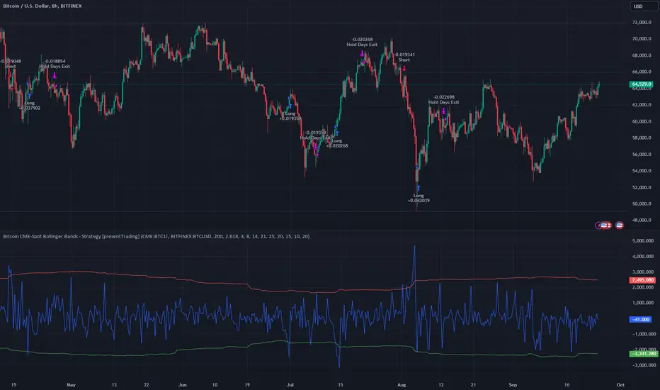
Bitcoin CME-Spot Z-Spread - Strategy [presentTrading]This time is a swing trading strategy! It measures the sentiment of the Bitcoin market through the spread of CME Bitcoin Futures and Bitfinex BTCUSD Spot prices. By applying Bollinger Bands to the spread, the strategy seeks to capture mean-reversion opportunities when prices deviate significantly from their historical norms
█ Introduction and How it is Different
The Bitcoin CME-Spot Bollinger Bands Strategy is designed to capture mean-reversion opportunities by exploiting the spread between CME Bitcoin Futures and Bitfinex BTCUSD Spot prices. The strategy uses Bollinger Bands to detect when the spread between these two correlated assets has deviated significantly from its historical norm, signaling potential overbought or oversold conditions.
What sets this strategy apart is its focus on spread trading between futures and spot markets rather than price-based indicators. By applying Bollinger Bands to the spread rather than individual prices, the strategy identifies price inefficiencies across markets, allowing traders to take advantage of the natural reversion to the mean that often occurs in these correlated assets.
BTCUSD 8hr Performance
█ Strategy, How It Works: Detailed Explanation
The strategy relies on Bollinger Bands to assess the volatility and relative deviation of the spread between CME Bitcoin Futures and Bitfinex BTCUSD Spot prices. Bollinger Bands consist of a moving average and two standard deviation bands, which help measure how much the spread deviates from its historical mean.
🔶 Spread Calculation:
The spread is calculated by subtracting the Bitfinex spot price from the CME Bitcoin futures price:
Spread = CME Price - Bitfinex Price
This spread represents the difference between the futures and spot markets, which may widen or narrow based on supply and demand dynamics in each market. By analyzing the spread, the strategy can detect when prices are too far apart (potentially overbought or oversold), indicating a trading opportunity.
🔶 Bollinger Bands Calculation:
The Bollinger Bands for the spread are calculated using a simple moving average (SMA) and the standard deviation of the spread over a defined period.
1. Moving Average (SMA):
The simple moving average of the spread (mu_S) over a specified period P is calculated as:
mu_S = (1/P) * sum(S_i from i=1 to P)
Where S_i represents the spread at time i, and P is the lookback period (default is 200 bars). The moving average provides a baseline for the normal spread behavior.
2. Standard Deviation:
The standard deviation (sigma_S) of the spread is calculated to measure the volatility of the spread:
sigma_S = sqrt((1/P) * sum((S_i - mu_S)^2 from i=1 to P))
3. Upper and Lower Bollinger Bands:
The upper and lower Bollinger Bands are derived by adding and subtracting a multiple of the standard deviation from the moving average. The number of standard deviations is determined by a user-defined parameter k (default is 2.618).
- Upper Band:
Upper Band = mu_S + (k * sigma_S)
- Lower Band:
Lower Band = mu_S - (k * sigma_S)
These bands provide a dynamic range within which the spread typically fluctuates. When the spread moves outside of these bands, it is considered overbought or oversold, potentially offering trading opportunities.
Local view
🔶 Entry Conditions:
- Long Entry: A long position is triggered when the spread crosses below the lower Bollinger Band, indicating that the spread has become oversold and is likely to revert upward.
Spread < Lower Band
- Short Entry: A short position is triggered when the spread crosses above the upper Bollinger Band, indicating that the spread has become overbought and is likely to revert downward.
Spread > Upper Band
🔶 Risk Management and Profit-Taking:
The strategy incorporates multi-step take profits to lock in gains as the trade moves in favor. The position is gradually reduced at predefined profit levels, reducing risk while allowing part of the trade to continue running if the price keeps moving favorably.
Additionally, the strategy uses a hold period exit mechanism. If the trade does not hit any of the take-profit levels within a certain number of bars, the position is closed automatically to avoid excessive exposure to market risks.
█ Trade Direction
The trade direction is based on deviations of the spread from its historical norm:
- Long Trade: The strategy enters a long position when the spread crosses below the lower Bollinger Band, signaling an oversold condition where the spread is expected to narrow.
- Short Trade: The strategy enters a short position when the spread crosses above the upper Bollinger Band, signaling an overbought condition where the spread is expected to widen.
These entries rely on the assumption of mean reversion, where extreme deviations from the average spread are likely to revert over time.
█ Usage
The Bitcoin CME-Spot Bollinger Bands Strategy is ideal for traders looking to capitalize on price inefficiencies between Bitcoin futures and spot markets. It’s especially useful in volatile markets where large deviations between futures and spot prices occur.
- Market Conditions: This strategy is most effective in correlated markets, like CME futures and spot Bitcoin. Traders can adjust the Bollinger Bands period and standard deviation multiplier to suit different volatility regimes.
- Backtesting: Before deployment, backtesting the strategy across different market conditions and timeframes is recommended to ensure robustness. Adjust the take-profit steps and hold periods to reflect the trader’s risk tolerance and market behavior.
█ Default Settings
The default settings provide a balanced approach to spread trading using Bollinger Bands but can be adjusted depending on market conditions or personal trading preferences.
🔶 Bollinger Bands Period (200 bars):
This defines the number of bars used to calculate the moving average and standard deviation for the Bollinger Bands. A longer period smooths out short-term fluctuations and focuses on larger, more significant trends. Adjusting the period affects the responsiveness of the strategy:
- Shorter periods (e.g., 100 bars): Makes the strategy more reactive to short-term market fluctuations, potentially generating more signals but increasing the risk of false positives.
- Longer periods (e.g., 300 bars): Focuses on longer-term trends, reducing the frequency of trades and focusing only on significant deviations.
🔶 Standard Deviation Multiplier (2.618):
The multiplier controls how wide the Bollinger Bands are around the moving average. By default, the bands are set at 2.618 standard deviations away from the average, ensuring that only significant deviations trigger trades.
- Higher multipliers (e.g., 3.0): Require a more extreme deviation to trigger trades, reducing trade frequency but potentially increasing the accuracy of signals.
- Lower multipliers (e.g., 2.0): Make the bands narrower, increasing the number of trade signals but potentially decreasing their reliability.
🔶 Take-Profit Levels:
The strategy has four take-profit levels to gradually lock in profits:
- Level 1 (3%): 25% of the position is closed at a 3% profit.
- Level 2 (8%): 20% of the position is closed at an 8% profit.
- Level 3 (14%): 15% of the position is closed at a 14% profit.
- Level 4 (21%): 10% of the position is closed at a 21% profit.
Adjusting these take-profit levels affects how quickly profits are realized:
- Lower take-profit levels: Capture gains more quickly, reducing risk but potentially cutting off larger profits.
- Higher take-profit levels: Let trades run longer, aiming for bigger gains but increasing the risk of price reversals before profits are locked in.
🔶 Hold Days (20 bars):
The strategy automatically closes the position after 20 bars if none of the take-profit levels are hit. This feature prevents trades from being held indefinitely, especially if market conditions are stagnant. Adjusting this:
- Shorter hold periods: Reduce the duration of exposure, minimizing risks from market changes but potentially closing trades too early.
- Longer hold periods: Allow trades to stay open longer, increasing the chance for mean reversion but also increasing exposure to unfavorable market conditions.
By understanding how these default settings affect the strategy’s performance, traders can optimize the Bitcoin CME-Spot Bollinger Bands Strategy to their preferences, adapting it to different market environments and risk tolerances.
Martingale + Grid DCA Strategy [YinYangAlgorithms]This Strategy focuses on strategically Martingaling when the price has dropped X% from your current Dollar Cost Average (DCA). When it does Martingale, it will create a Purchase Grid around this location to likewise attempt to get you a better DCA. Likewise following the Martingale strategy, it will sell when your Profit has hit your target of X%.
Martingale may be an effective way to lower your DCA. This is due to the fact that if your initial purchase; or in our case, initial Grid, all went through and the price kept going down afterwards, that you may purchase more to help lower your DCA even more. By doing so, you may bring your DCA down and effectively may make it easier and quicker to reach your target profit %.
Grid trading may be an effective way of reducing risk and lowering your DCA as you are spreading your purchases out over multiple different locations. Likewise we offer the ability to ‘Stack Grids’. What this means, is that if a single bar was to go through 20 grids, the purchase amount would be 20x what each grid is valued at. This may help get you a lower DCA as rather than creating 20 purchase orders at each grid location, we create a single purchase order at the lowest grid location, but for 20x the amount.
By combining both Martingale and Grid DCA techniques we attempt to lower your DCA strategically until you have reached your target profit %.
Before we start, we just want to make it known that first off, this Strategy features 8% Commission Fees, you may change this in the Settings to better reflect the Commission Fees of your exchange. On a similar note, due to Commission Fees being one of the number one profit killers in fast swing trade strategies, this strategy doesn’t focus on low trades, but the ideology of it may result in low amounts of trades. Please keep in mind this is not a bad thing. Since it has the ability to ‘Stack Grid Purchases’ it may purchase more for less and result in more profit, less commission fees, and likewise less # of trades.
Tutorial:
In this example above, we have it set so we Martingale twice, and we use 100 grids between the upper and lower level of each martingale; for a total of 200 Grids. This strategy will take total capital (initial capital + net profit) and divide it by the amount of grids. This will result in the $ amount purchased per grid. For instance, say you started with $10,000 and you’ve made $2000 from this Strategy so far, your total capital is $12,000. If you likewise are implementing 200 grids within your Strategy, this will result in $12,000 / 200 = $60 per grid. However, please note, that the further down the grid / martingale is, the more volume it is able to purchase for $60.
The white line within the Strategy represents your DCA. As the Strategy makes purchases, this will continue to get lower as will your Target Profit price (Blue Line). When the Close goes above your Target Profit price, the Strategy will close all open positions and claim the profit. This profit is then reinvested back into the Strategy, which may exponentially help the Strategy become more profitable the longer it runs for.
In the example above, we’ve zoomed in on the first example. In this we want to focus on how the Strategy got back into the trades shortly after it sold. Currently within the Settings we have it set so our entry is when the Lowest with a length of 3 is less than the previous Lowest with a length of 3. This is 100% customizable and there are multiple different entry options you can choose from and customize such as:
EMA 7 Crossover EMA 21
EMA 7 Crossunder EMA 21
RSI 14 Crossover RSI MA 14
RSI 14 Crossunder RSI MA 14
MFI 14 Crossover MFI MA 14
MFI 14 Crossunder MFI MA 14
Lowest of X Length < Previous Lowest of X Length
Highest of X Length > Previous Highest of X Length
All of these entry options may be tailored to be checked for on a different Time Frame than the one you are currently using the Strategy on. For instance, you may be running the Strategy on the 15 minute Time Frame yet decide you want the RSI to cross over the RSI MA on the 1 Day to be a valid entry location.
Please keep in mind, this Strategy focuses on DCA, this means you may not want the initial purchase to be the best location. You may want to buy when others think it is a good time to sell. This is because there may be strong bearish momentum which drives the price down drastically and potentially getting you a good DCA before it corrects back up.
We will continue to add more Entry options as time goes on, and if you have any in mind please don’t hesitate to let us know.
Now, back to the example above, if we refer to the Yellow circle, you may see that the Lowest of a length of 3 was less than its previous lowest, this triggered the martingales to create their grids. Only a few bars later, the price went into the first grid and went a little lower than its midpoint (Yellow line). This caused about 60% of the first grid to be purchased. Shortly after the price went even lower into this grid and caused the entire first martingale grid to be purchased. However, if you notice, the white line (your DCA) is lower than the midpoint of the first grid. This is due to the fact that we have ‘Stack Grid Purchases’ enabled. This allows the Strategy to purchase more when a single bar crosses through multiple grid locations; and effectively may lower your average more than if it simply executed a purchase order at each grid.
Still looking at the same location within our next example, if we simply increase the Martingale amount from 2 to 3 we can see something strange happens. What happened is our Target Profit price was reached, then our entry condition was met, which caused all of the martingale grids to be formed; however, the price continued to increase afterwards. This may not be a good thing, sure the price could correct back down to these grid locations, but what if it didn’t and it just kept increasing? This would result in this Strategy being stuck and unable to make any trades. For this reason we have implemented a Failsafe in the Settings called ‘Reset Grids if no purchase happens after X bars’.
We have enabled our Failsafe ‘Reset Grids if no purchase happens after X bars’ in this example above. By default it is set to 100 bars, but you can change this to whatever works best for you. If you set it to 0, this Failsafe will be disabled and act like the example prior where it is possible to be stuck with no trades executing.
This Failsafe may be an important way to ensure the Strategy is able to make purchases, however it may also mean the Grids increase in price when it is used, and if a massive correction were to occur afterwards, you may lose out on potential profit.
This Strategy was designed with WebHooks in mind. WebHooks allow you to send signals from the Strategy to your exchange. Simply set up a Custom TradingView Bot within the OKX exchange or 3Commas platform (which has your exchange API), enter the data required from the bot into the settings here, select your bot type in ‘Webhook Alert Type’, and then set up the alert. After that you’re good to go and this Strategy will fully automate all of its trades within your exchange for you. You need to format the Alert a certain way for it to work, which we will go over in the next example.
Add an alert for this Strategy and simply modify the alert message so all it says is:
{{strategy.order.alert_message}}
Likewise change from the Alert ‘Settings’ to Alert ‘Notifications’ at the top of the alert popup. Within the Notifications we will enable ‘Webhook URL’ and then we will pass the URL we are sending the Webhook to. In this example we’ve put OKX exchange Webhook URL, however if you are using 3Commas you’ll need to change this to theirs.
OKX Webhook URL:
www.okx.com
3Commas Webhook URL:
app.3commas.io
Make sure you click ‘Create’ to actually create this alert. After that you’re all set! There are many Tutorials videos you can watch if you are still a little confused as to how Webhook trading works.
Due to the nature of this Strategy and how it is designed to work, it has the ability to never sell unless there it will make profit. However, because of this it also may be stuck waiting in trades for quite a long period of time (usually a few months); especially when your Target Profit % is 15% like in the example above. However, this example above may be a good indication that it may maintain profitability for a long period of time; considering this ‘Deep Backtest’ is from 2017-8-17.
We will conclude the tutorial here. Hopefully you understand how this Strategy has the potential to make calculated and strategic DCA Grid purchases for you and then based on a traditional Martingale fashion, bulk sell at the desired Target Profit Percent.
Settings:
Purchase Settings:
Only Purchase if its lower than DCA: Generally speaking, we want to lower our Average, and therefore it makes sense to only buy when the close is lower than our current DCA and a Purchase Condition is met.
Purchase Condition: When creating the initial buy location you must remember, you want to Buy when others are Fearful and Sell when others are Greedy. Therefore, many of the Buy conditions involve times many would likewise Sell. This is one of the bonuses to using a Strategy like this as it will attempt to get you a good entry location at times people are selling.
Lower / Upper Change Length: This Lower / Upper Length is only used if the Purchase Condition is set to 'Lower Changed' or 'Upper Changed'. This is when the Lowest or Highest of this length changes. Lowest would become lower or Highest would become higher.
Purchase Resolution: Purchase Resolution is the Time Frame that the Purchase Condition is calculated on. For instance, you may only want to start a new Purchase Order when the RSI Crosses RSI MA on the 1 Day, but yet you run this Strategy on the 15 minutes.
Sell Settings:
Trailing Take Profit: Trailing Take Profit is where once your Target Profit Percent has been hit, this will trail up to attempt to claim even more profit.
Target Profit Percent: What is your Target Profit Percent? The Strategy will close all positions when the close price is greater than your DCA * this Target Profit Percent.
Grid Settings:
Stack Grid Purchases: If a close goes through multiple Buy Grids in one bar, should we amplify its purchase amount based on how many grids it went through?
Reset Grids if no purchase happens after X Bars: Set this to 0 if you never want to reset. This is very useful in case the price is very bullish and continues to increase after our Target Profit location is hit. What may happen is, Target Profit location is hit, then the Entry condition is met but the price just keeps increasing afterwards. We may not want to be sitting waiting for the price to drop, which may never happen. This is more of a failsafe if anything. You may set it very large, like 500+ if you only want to use it in extreme situations.
Grid % Less than Initial Purchase Price: How big should our Buy Grid be? For instance if we bought at 0.25 and this value is set to 20%, that means our Buy Grid spans from 0.2 - 0.25.
Grid Amounts: How many Grids should we create within our Buy location?
Martingale Settings:
Amount of Times 'Planned' to Martingale: The more Grids + the More Martingales = the less $ spent per grid, however the less risk. Remember it may be better to be right and take your time than risk too much and be stuck too long.
Martingale Percent: When the current price is this percent less than our DCA, lets create another Buy Grid so we can lower our average more. This will make our profit location less.
Webhook Alerts:
Webhook Alert Type: How should we format this Alert? 3Commas and OKX take their alerts differently, so please select the proper one or your webhooks won't work.
3Commas Webhook Alerts:
3Commas Bot ID: The 3Commas Bot ID is needed so we know which BOT ID we are sending this webhook too.
3Commas Email Token: The 3Commas Email Token is needed for your webhooks to work properly as it is linked to your account.
OKX Webhook Alerts:
OKX Signal Token: This Signal Token is attached to your OKX bot and will be used to access it within OKX.
If you have any questions, comments, ideas or concerns please don't hesitate to contact us.
HAPPY TRADING!

GKD-BT Baseline Backtest [Loxx]The Giga Kaleidoscope GKD-BT Baseline Backtest is a backtesting module included in Loxx's "Giga Kaleidoscope Modularized Trading System."
█ GKD-BT Baseline Backtest
The GKD-BT Baseline Backtest allows traders to backtest the Regular and Stepped baselines used in the GKD trading system. This module includes 65+ moving averages and 15+ types of volatility to choose from.
Additionally, this backtest module provides the option to test the GKD-B indicator with 1 to 3 take profits and 1 stop loss. The Trading backtest allows for the use of 1 to 3 take profits, while the Full backtest is limited to 1 take profit. The Trading backtest also offers the capability to apply a trailing take profit.
In terms of the percentage of trade removed at each take profit, this backtest module has the following hardcoded values:
Take profit 1: 50% of the trade is removed
Take profit 2: 25% of the trade is removed
Take profit 3: 25% of the trade is removed
Stop loss: 100% of the trade is removed
After each take profit is achieved, the stop loss level is adjusted. When take profit 1 is reached, the stop loss is moved to the entry point. Similarly, when take profit 2 is reached, the stop loss is shifted to take profit 1. The trailing take profit feature comes into play after take profit 2 or take profit 3, depending on the number of take profits selected in the settings. The trailing take profit is always activated on the final take profit when 2 or more take profits are chosen.
The backtest also offers the capability to restrict by a specific date range, allowing for simulated forward testing based on past data. Additionally, users have the option to display or hide a trading panel that provides relevant information about the backtest, statistics, and the current trade. It is also possible to activate alerts and toggle sections of the trading panel on or off. On the chart, historical take profit and stop loss levels are represented by horizontal lines overlaid for reference.
This backtest also includes an optional GKD-E Exit indicator that can be used to test early exits.
The GKD system utilizes volatility-based take profits and stop losses. Each take profit and stop loss is calculated as a multiple of volatility. You can change the values of the multipliers in the settings as well.
To utilize this strategy, follow these steps:
1. (Required) Import the value "Input into NEW GKD-BT Backtest" from the GKD-B Baseline indicator into the GKD-BT Baseline Backtest field "Import GKD-B Baseline"
2. (Optional) Import the value "Input into NEW GKD-BT Backtest" from the GKD-E Exit indicator into the GKD-BT Baseline Backtest field "Import GKD-E Exit". You can toggle the Exit on or off using the "Activate GKD-E Exit" option.
Baselines that are compatible with this backtest module:
GKD-B Baseline
GKD-B Stepped Baseline
Volatility Types Included
17 types of volatility are included in this indicator
Close-to-Close
Parkinson
Garman-Klass
Rogers-Satchell
Yang-Zhang
Garman-Klass-Yang-Zhang
Exponential Weighted Moving Average
Standard Deviation of Log Returns
Pseudo GARCH(2,2)
Average True Range
True Range Double
Standard Deviation
Adaptive Deviation
Median Absolute Deviation
Efficiency-Ratio Adaptive ATR
Mean Absolute Deviation
Static Percent
█ Giga Kaleidoscope Modularized Trading System
Core components of an NNFX algorithmic trading strategy
The NNFX algorithm is built on the principles of trend, momentum, and volatility. There are six core components in the NNFX trading algorithm:
1. Volatility - price volatility; e.g., Average True Range, True Range Double, Close-to-Close, etc.
2. Baseline - a moving average to identify price trend
3. Confirmation 1 - a technical indicator used to identify trends
4. Confirmation 2 - a technical indicator used to identify trends
5. Continuation - a technical indicator used to identify trends
6. Volatility/Volume - a technical indicator used to identify volatility/volume breakouts/breakdown
7. Exit - a technical indicator used to determine when a trend is exhausted
8. Metamorphosis - a technical indicator that produces a compound signal from the combination of other GKD indicators*
*(not part of the NNFX algorithm)
What is Volatility in the NNFX trading system?
In the NNFX (No Nonsense Forex) trading system, ATR (Average True Range) is typically used to measure the volatility of an asset. It is used as a part of the system to help determine the appropriate stop loss and take profit levels for a trade. ATR is calculated by taking the average of the true range values over a specified period.
True range is calculated as the maximum of the following values:
-Current high minus the current low
-Absolute value of the current high minus the previous close
-Absolute value of the current low minus the previous close
ATR is a dynamic indicator that changes with changes in volatility. As volatility increases, the value of ATR increases, and as volatility decreases, the value of ATR decreases. By using ATR in NNFX system, traders can adjust their stop loss and take profit levels according to the volatility of the asset being traded. This helps to ensure that the trade is given enough room to move, while also minimizing potential losses.
Other types of volatility include True Range Double (TRD), Close-to-Close, and Garman-Klass
What is a Baseline indicator?
The baseline is essentially a moving average, and is used to determine the overall direction of the market.
The baseline in the NNFX system is used to filter out trades that are not in line with the long-term trend of the market. The baseline is plotted on the chart along with other indicators, such as the Moving Average (MA), the Relative Strength Index (RSI), and the Average True Range (ATR).
Trades are only taken when the price is in the same direction as the baseline. For example, if the baseline is sloping upwards, only long trades are taken, and if the baseline is sloping downwards, only short trades are taken. This approach helps to ensure that trades are in line with the overall trend of the market, and reduces the risk of entering trades that are likely to fail.
By using a baseline in the NNFX system, traders can have a clear reference point for determining the overall trend of the market, and can make more informed trading decisions. The baseline helps to filter out noise and false signals, and ensures that trades are taken in the direction of the long-term trend.
What is a Confirmation indicator?
Confirmation indicators are technical indicators that are used to confirm the signals generated by primary indicators. Primary indicators are the core indicators used in the NNFX system, such as the Average True Range (ATR), the Moving Average (MA), and the Relative Strength Index (RSI).
The purpose of the confirmation indicators is to reduce false signals and improve the accuracy of the trading system. They are designed to confirm the signals generated by the primary indicators by providing additional information about the strength and direction of the trend.
Some examples of confirmation indicators that may be used in the NNFX system include the Bollinger Bands, the MACD (Moving Average Convergence Divergence), and the MACD Oscillator. These indicators can provide information about the volatility, momentum, and trend strength of the market, and can be used to confirm the signals generated by the primary indicators.
In the NNFX system, confirmation indicators are used in combination with primary indicators and other filters to create a trading system that is robust and reliable. By using multiple indicators to confirm trading signals, the system aims to reduce the risk of false signals and improve the overall profitability of the trades.
What is a Continuation indicator?
In the NNFX (No Nonsense Forex) trading system, a continuation indicator is a technical indicator that is used to confirm a current trend and predict that the trend is likely to continue in the same direction. A continuation indicator is typically used in conjunction with other indicators in the system, such as a baseline indicator, to provide a comprehensive trading strategy.
What is a Volatility/Volume indicator?
Volume indicators, such as the On Balance Volume (OBV), the Chaikin Money Flow (CMF), or the Volume Price Trend (VPT), are used to measure the amount of buying and selling activity in a market. They are based on the trading volume of the market, and can provide information about the strength of the trend. In the NNFX system, volume indicators are used to confirm trading signals generated by the Moving Average and the Relative Strength Index. Volatility indicators include Average Direction Index, Waddah Attar, and Volatility Ratio. In the NNFX trading system, volatility is a proxy for volume and vice versa.
By using volume indicators as confirmation tools, the NNFX trading system aims to reduce the risk of false signals and improve the overall profitability of trades. These indicators can provide additional information about the market that is not captured by the primary indicators, and can help traders to make more informed trading decisions. In addition, volume indicators can be used to identify potential changes in market trends and to confirm the strength of price movements.
What is an Exit indicator?
The exit indicator is used in conjunction with other indicators in the system, such as the Moving Average (MA), the Relative Strength Index (RSI), and the Average True Range (ATR), to provide a comprehensive trading strategy.
The exit indicator in the NNFX system can be any technical indicator that is deemed effective at identifying optimal exit points. Examples of exit indicators that are commonly used include the Parabolic SAR, the Average Directional Index (ADX), and the Chandelier Exit.
The purpose of the exit indicator is to identify when a trend is likely to reverse or when the market conditions have changed, signaling the need to exit a trade. By using an exit indicator, traders can manage their risk and prevent significant losses.
In the NNFX system, the exit indicator is used in conjunction with a stop loss and a take profit order to maximize profits and minimize losses. The stop loss order is used to limit the amount of loss that can be incurred if the trade goes against the trader, while the take profit order is used to lock in profits when the trade is moving in the trader's favor.
Overall, the use of an exit indicator in the NNFX trading system is an important component of a comprehensive trading strategy. It allows traders to manage their risk effectively and improve the profitability of their trades by exiting at the right time.
What is an Metamorphosis indicator?
The concept of a metamorphosis indicator involves the integration of two or more GKD indicators to generate a compound signal. This is achieved by evaluating the accuracy of each indicator and selecting the signal from the indicator with the highest accuracy. As an illustration, let's consider a scenario where we calculate the accuracy of 10 indicators and choose the signal from the indicator that demonstrates the highest accuracy.
The resulting output from the metamorphosis indicator can then be utilized in a GKD-BT backtest by occupying a slot that aligns with the purpose of the metamorphosis indicator. The slot can be a GKD-B, GKD-C, or GKD-E slot, depending on the specific requirements and objectives of the indicator. This allows for seamless integration and utilization of the compound signal within the GKD-BT framework.
How does Loxx's GKD (Giga Kaleidoscope Modularized Trading System) implement the NNFX algorithm outlined above?
Loxx's GKD v2.0 system has five types of modules (indicators/strategies). These modules are:
1. GKD-BT - Backtesting module (Volatility, Number 1 in the NNFX algorithm)
2. GKD-B - Baseline module (Baseline and Volatility/Volume, Numbers 1 and 2 in the NNFX algorithm)
3. GKD-C - Confirmation 1/2 and Continuation module (Confirmation 1/2 and Continuation, Numbers 3, 4, and 5 in the NNFX algorithm)
4. GKD-V - Volatility/Volume module (Confirmation 1/2, Number 6 in the NNFX algorithm)
5. GKD-E - Exit module (Exit, Number 7 in the NNFX algorithm)
6. GKD-M - Metamorphosis module (Metamorphosis, Number 8 in the NNFX algorithm, but not part of the NNFX algorithm)
(additional module types will added in future releases)
Each module interacts with every module by passing data to A backtest module wherein the various components of the GKD system are combined to create a trading signal.
That is, the Baseline indicator passes its data to Volatility/Volume. The Volatility/Volume indicator passes its values to the Confirmation 1 indicator. The Confirmation 1 indicator passes its values to the Confirmation 2 indicator. The Confirmation 2 indicator passes its values to the Continuation indicator. The Continuation indicator passes its values to the Exit indicator, and finally, the Exit indicator passes its values to the Backtest strategy.
This chaining of indicators requires that each module conform to Loxx's GKD protocol, therefore allowing for the testing of every possible combination of technical indicators that make up the six components of the NNFX algorithm.
What does the application of the GKD trading system look like?
Example trading system:
Backtest: GKD-BT Baseline Backtest as shown on the chart above
Baseline: Hull Moving Average as shown on the chart above
Volatility/Volume: Hurst Exponent
Confirmation 1: Sherif's HiLo
Confirmation 2: uf2018
Continuation: Coppock Curve
Exit: Fisher Transform as shown on the chart above
Metamorphosis: Baseline Optimizer
Each GKD indicator is denoted with a module identifier of either: GKD-BT, GKD-B, GKD-C, GKD-V, GKD-M, or GKD-E. This allows traders to understand to which module each indicator belongs and where each indicator fits into the GKD system.
█ Giga Kaleidoscope Modularized Trading System Signals
Standard Entry
1. GKD-C Confirmation gives signal
2. Baseline agrees
3. Price inside Goldie Locks Zone Minimum
4. Price inside Goldie Locks Zone Maximum
5. Confirmation 2 agrees
6. Volatility/Volume agrees
1-Candle Standard Entry
1a. GKD-C Confirmation gives signal
2a. Baseline agrees
3a. Price inside Goldie Locks Zone Minimum
4a. Price inside Goldie Locks Zone Maximum
Next Candle
1b. Price retraced
2b. Baseline agrees
3b. Confirmation 1 agrees
4b. Confirmation 2 agrees
5b. Volatility/Volume agrees
Baseline Entry
1. GKD-B Baseline gives signal
2. Confirmation 1 agrees
3. Price inside Goldie Locks Zone Minimum
4. Price inside Goldie Locks Zone Maximum
5. Confirmation 2 agrees
6. Volatility/Volume agrees
7. Confirmation 1 signal was less than 'Maximum Allowable PSBC Bars Back' prior
1-Candle Baseline Entry
1a. GKD-B Baseline gives signal
2a. Confirmation 1 agrees
3a. Price inside Goldie Locks Zone Minimum
4a. Price inside Goldie Locks Zone Maximum
5a. Confirmation 1 signal was less than 'Maximum Allowable PSBC Bars Back' prior
Next Candle
1b. Price retraced
2b. Baseline agrees
3b. Confirmation 1 agrees
4b. Confirmation 2 agrees
5b. Volatility/Volume agrees
Volatility/Volume Entry
1. GKD-V Volatility/Volume gives signal
2. Confirmation 1 agrees
3. Price inside Goldie Locks Zone Minimum
4. Price inside Goldie Locks Zone Maximum
5. Confirmation 2 agrees
6. Baseline agrees
7. Confirmation 1 signal was less than 7 candles prior
1-Candle Volatility/Volume Entry
1a. GKD-V Volatility/Volume gives signal
2a. Confirmation 1 agrees
3a. Price inside Goldie Locks Zone Minimum
4a. Price inside Goldie Locks Zone Maximum
5a. Confirmation 1 signal was less than 'Maximum Allowable PSVVC Bars Back' prior
Next Candle
1b. Price retraced
2b. Volatility/Volume agrees
3b. Confirmation 1 agrees
4b. Confirmation 2 agrees
5b. Baseline agrees
Confirmation 2 Entry
1. GKD-C Confirmation 2 gives signal
2. Confirmation 1 agrees
3. Price inside Goldie Locks Zone Minimum
4. Price inside Goldie Locks Zone Maximum
5. Volatility/Volume agrees
6. Baseline agrees
7. Confirmation 1 signal was less than 7 candles prior
1-Candle Confirmation 2 Entry
1a. GKD-C Confirmation 2 gives signal
2a. Confirmation 1 agrees
3a. Price inside Goldie Locks Zone Minimum
4a. Price inside Goldie Locks Zone Maximum
5a. Confirmation 1 signal was less than 'Maximum Allowable PSC2C Bars Back' prior
Next Candle
1b. Price retraced
2b. Confirmation 2 agrees
3b. Confirmation 1 agrees
4b. Volatility/Volume agrees
5b. Baseline agrees
PullBack Entry
1a. GKD-B Baseline gives signal
2a. Confirmation 1 agrees
3a. Price is beyond 1.0x Volatility of Baseline
Next Candle
1b. Price inside Goldie Locks Zone Minimum
2b. Price inside Goldie Locks Zone Maximum
3b. Confirmation 1 agrees
4b. Confirmation 2 agrees
5b. Volatility/Volume agrees
Continuation Entry
1. Standard Entry, 1-Candle Standard Entry, Baseline Entry, 1-Candle Baseline Entry, Volatility/Volume Entry, 1-Candle Volatility/Volume Entry, Confirmation 2 Entry, 1-Candle Confirmation 2 Entry, or Pullback entry triggered previously
2. Baseline hasn't crossed since entry signal trigger
4. Confirmation 1 agrees
5. Baseline agrees
6. Confirmation 2 agrees
Easy Trade Pro [Buy and Sell Strategy + Backtesting System]Hello Traders,
Easy Trade Pro is a comprehensive tool that combines multiple technical indicators into a single customizable one. This tool is the culmination of an extensive trading career, it is designed to help traders navigate the markets in any timeframe and financial asset, like Equities, Futures, Crypto, Forex and Commodities.
Before we deep dive into the comprehensive guide on what Easy Trade Pro is, let's kick off by showcasing the strategy used in this example. Please note, we have adopted an extremely conservative approach strictly following the Tradingview House Rules, which you can review here: www.tradingview.com
The backtest strategy parameters:
Currency pair: EUR USD
Timeframe: 15-min chart
Market: Spot, no leverage
Broker: FXCM
Trading range: 2022-09-01 07:30 — 2023-06-26 20:00
Backtesting range: 2022-08-31 23:00 — 2023-06-26 20:00
Initial Capital: $10,000
Buy Order Size: 20% of the capital, $2,000
Stop Loss: 0.50%
Sell orders: Four different take profits where we unload the position by 25% each time
Broker Fees: Commission set at 0.08$
Slippage: 10 ticks
Understanding FXCM Commissions and Setting Realistic Slippage for EUR/USD Spot Trading:
◉I would like to provide some clarity on the commission structure and slippage setting used in the study for trading the EUR/USD pair on the FXCM spot market. Based on the information available, FXCM charges a commission of $4.00 per standard lot (100,000) on both sides of the trade (meaning at open and close) for the EUR/USD pair. Since the study involve an order size of $2,000 USD, which is equivalent to 0.02 lots, the commission fee for one side of the trade (either buying or selling) would be calculated as $4.00 multiplied by 0.02, which is $0.08. This means that for each individual trade, whether it be a buy or sell, the commission fee would be $0.08.
◉As for slippage, it is crucial to account for the inherent uncertainty in the execution price due to market fluctuations. In the forex market, the EUR/USD pair is quoted with a precision of five decimal places, with the smallest price change being a "pipette" (0.00001). Given that slippage can vary based on market conditions, it is considered fair practice to use a slippage of around 10 ticks under normal market conditions for the EUR/USD pair. This allows for a more realistic representation of the execution price, especially in a liquid and fast-moving market such as forex.
More detailed information about FXCM fees structure in the link below:
docs.fxcorporate.com
Enter a Trade conditions:
For our buy order, we utilize a custom buy signal called 'Bullish Reversal'. A detailed explanation of this and other buy orders can be found later in the guide, specifically in section 1).
To enhance realism in our trading strategy, we have implemented a confirmation mechanism. When utilizing the strategy tester, you have the option to input a value to determine the number of confirmation candles to consider.
For example, if you set the input to 1, the system will check if the next candle following the signal meets the criteria for confirmation. If set to 2, the system will evaluate the second candle, and so on for higher values. The confirmation is determined by comparing the closing or opening price of the selected buy signal candle with the corresponding closing price of the confirmation candle.
In this case we choose as buy signal: 'Bullish Reversal' + 2 candle of confirmation
Exit a trade conditions:
On the sell side, we exit a trade in four different types of sell orders where we take profits. Inside '', you will encounter unique labels attributed to our custom sell signals. A detailed explanation of these sell orders can be found later in the guide, specifically in section 1). We used custom order called:
1TP 'Good Sell'
2TP 'Good Sell'
3TP 'Good Sell'
4TP 'Bearish Reversal' + 4 confirmation candles
Our confirmation logic, for sell signals, is applied only to 'Bearish Reversal' signal. The confirmation is determined by comparing the closing or opening price of the selected 'Bearish Reversal' candle with the corresponding closing price of the confirmation candle. In this case, we wait for the fourth candle from the 'Bearish Reversal' signal to confirm the sell trade.
Protect your capital:
This super-conservative study involves a clear low risk, with the use of $2,000, 20% of our capital. If the stop loss of 0.5% were triggered, we lose 10$, equating to 0.10% of $10,000 - thus affecting only 0.10% of our capital.
Super Conservative Approach & Results:
With 353 closed trades, we achieved a net profit of 2.03%, or $203.34$ relative to our initial $10,000 capital, and a win rate of 73.37%.
Less Conservative Approach & Results:
We could also consider increasing our risk to 0.5% of our capital per trade. We would maintain our stop loss at 0.50%, but we would need to use all our capital to enter the market. If the stop loss of 0.5% will be triggered, we would lose 50$, equating to 0.5% of $10,000.
In this scenario, our net profit would have increased to 10.15%, equivalent to $1015.
Please be aware:
While fully automated strategies can bring considerable advantages, they are not without their cons. For one, relying solely on an automated system may not take into account the potential confluence of other strategies or indicators, such as the significance of support and resistance zones. These elements often require a more nuanced, human understanding of the markets and cannot always be perfectly replicated by an algorithm.
Additionally, it's essential to remember that a significant percentage of traders are not consistently profitable. As such, prudent risk management, a conservative approach, and acceptance of a reasonable profit are crucial aspects of successful trading. While the allure of high returns can be tempting, the sustainability of your trading strategy should always take precedence. Achieving steady, reliable profits over time often outweighs the appeal of a risky, high-return strategy that could potentially lead to substantial losses.
So, while automation can be a powerful tool in your trading arsenal, it's also important to consider other strategies and factors. Always ensure you're managing your risk effectively and approaching trading with a realistic and informed perspective.
------------------------------------------------------------------------ Why Easy Trade Pro is Original? ----------------------------------------------------------------------------------
We developed Easy Trade Pro as a unique and comprehensive solution, and we decided to protect our code to preserve its originality. We invested significant time and effort into making it a realistic trading strategy simulator. The standout features that set Easy Trade Pro apart include:
☀ Versatile Stop Loss Mechanisms: Stop loss execution can be complex and often requires careful coding to work as intended. In most freely available open-source codes, stop losses are implemented using the Average True Range (ATR). ATR can be beneficial but has limitations:
☁ Lagging Indicator - Like most technical indicators, the ATR is a lagging indicator. This means it is based on past data, and so it may not accurately reflect future market volatility. If market conditions change rapidly, the ATR may not adjust quickly enough, potentially leading to suboptimal stop loss levels.
☁ No Directional Information - The ATR measures volatility, but it does not provide any indication of the direction of the trend. Therefore, it should not be used as a standalone tool for making trading decisions, but should be used in conjunction with other technical analysis tools that can provide directional cues.
☁ Inefficiency in Trending Markets - In strongly trending markets, ATR-based stops can sometimes be too far from the current price level. This could lead to larger losses if the price moves against your trade before hitting the stop loss. On the flip side, in less volatile, sideways markets, an ATR-based stop might be set too close to the entry point, leading to premature stop outs.
☁ Overoptimization Risk - If you're backtesting a trading strategy, there's a risk of overoptimizing your stop loss settings by fine-tuning them to past data. The best ATR multiplier that worked in the past might not necessarily work in the future, leading to potential performance issues.
☀ We countered these by implementing four different types of 'protect the trade' mechanisms:
✔ Fixed Percentage Stop Loss
✔ Trailing Stop Loss
✔ Stop Loss Moved to Entry Upon Reaching Certain Gain
✔ Stop Loss Moved to Entry Upon Reaching First Take Profit Order ("Custom Order").
☀ Dual Exit Strategy: We incorporated two distinct methods of exiting a trade. The first uses our custom signals, while the second triggers exit at a certain percentage of gain.
☀ Multiple Take Profit Orders: You have the flexibility to establish up to four different sell orders. This feature enables you to fractionate your exit strategy according to your needs. You can choose to trigger these fractions based on our custom signals or determine your own exit points by setting targeted gains at a fixed percentage.
☀ Confirmation Candle System: This feature enhances trade precision by requiring confirmation candles after a buy or sell signal. This confirmation, dependent on the next candle's closing price, helps reduce false signals and improves entry and exit points. While our confirmation system is applicable to all custom buy signals, it's solely dedicated for the bearish reversal when it comes to sell signals.
☀ Universal Compatibility: Easy Trade Pro's Strategy Tester works perfectly with any asset class. The code can handle different contract types, including the SPX contracts and fractional assets like Bitcoin. It's optimized to ensure proper execution of trades without rounding issues.
☀ Bullish and Bearish Reversal candles: Our method of detecting these pivotal candles combines conditions from buy and sell signals with pertinent divergences in Price, RSI, and Volume (OBV). The distinguishing factor, however, lies in recognizing significant shifts in market structure and liquidity grabs. To further enhance the credibility of our indicator, we've incorporated Bollinger Bands, serving as an additional layer in spotting potential trend reversals, particularly when aligned with long-wick candlesticks, engulfing patterns, and morning or evening star formations.
☀ Non-Repainting Indicator: Our indicator signals are designed not to repaint. Once a signal appears, it stays fixed, offering a reliable tool for your trading decisions.
================================================== EXTENSIVE TECHNICAL DESCRIPTION ====================================================
Easy Trade Pro is versatile, allowing you to analyze market trends across any financial asset. With its rigorous testing, our tool can be used confidently on any timeframe, from 1D to 1min, whether you prefer longer-term or shorter-term trades.
Although we recommend trading on timeframes between 1D and 1min, higher timeframes like 1W chart, can also provide broader insights.
Our study combines a variety of popular technical indicators, such as RSI, Stochastic RSI, MACD, DMI, Bollinger Bands as well as relevant EMAs. On the volume side OBV and MFI. Using a data-driven approach, “Easy Trade Pro” analyzes historical market trends to identify optimal ways to combine these indicators with significant divergences between price and oscillators. On top of that the code considers relevant changes in market structure and liquidity grabs, to generate reliable and accurate signals for potential buy and sell opportunities.
* ☎ --> Please not that MACD, BBs, and EMAs account for a minimal part of our script <--- ☎, If you're looking for a simpler tool, consider checking out our open-source indicator, 'RSI, SRSI, MACD, and DMI cross - Open source code'. You can find it here:
With our customizable system, traders will be able to identify:
1) Three types of buy signals🐂,💰,💎 and sell signals 🐻,🔨,💀
2) Bullish and bearish reversal candles with support and resistance lines
3) Bull and bear momentum signals
4) A function that utilizes Color bars to identify the strength of the trend
5) Three customizable moving averages
6) Alerts direct to your email or phone
7) Advanced and customizable settings menu
8) Our software also includes a backtesting system that that allows users to test their trading strategies on historical data, to check how they would have performed in real-world market conditions. This can help refine a trading strategy and make more informed decisions.
------------------------------------------------------------------------------ 1) BUY AND SELL SIGNALS ---------------------------------------------------------------------------------
Our buy and sell signals are generated using a custom combination of RSI, MFI, and Stochastic RSI levels, as well as relevant MACD and Stochastic RSI crosses. These indicators are carefully analyzed to identify potential trading opportunities and determine optimal entry and exit points for trades.
RSI (Relative strength index) measures the strength of a security's price action, while the SRSI (Stochastic Relative Strength Index) is a momentum oscillator that measures the current price relative to its high and low range over a set period. The Money Flow Index (MFI) is another momentum indicator that uses both price and volume data to measure buying and selling pressure. MACD (Moving Average Convergence Divergence) is a popular technical indicator used in financial markets to analyze price trends and momentum.
▶ With our system, you'll be able to identify three different levels of buy signals:
◉ The first level of buy signal is represented by a 🐂 emoji and is a "Good Buy". This signal indicates a possible buying opportunity. It indicates that could be a good opportunity to enter in a long trade. It's important to note that, the "Good Buy" signal can sometimes be supplemented with a green "Bull" text and a flag plotshape positioned beneath the signal. In these scenarios, we categorize this as a "Good Buy Bull" signal.
◉ The second level of buy signal is represented by a 💰 emoji and is a "Great Buy". This signal indicates a stronger buying opportunity than the "Good Buy" signal.
◉ The third and strongest buy signal is represented by a 💎 emoji and is an "Incredible Buy". This signal indicates a stronger buying opportunity than the "Good Buy" and "Great Buy" signals
▶ With our system, you'll be able to identify three different levels of sell signals:
◉ On the sell side, the first level is represented by a 🐻 emoji and is a "Good Sell". This signal indicates a possible selling opportunity. It indicates that could be a good opportunity to exit a trade or open a short position. It's important to note that, the "Good Sell" signal can occasionally be accompanied by a red "Bear" text and a flag plotshape positioned beneath the signal. In such instances, we refer to this as a "Good Sell Bear" signal.
◉ The second sell signal is represented by a 🔨 emoji and is a "Great Sell". This signal indicates a stronger selling opportunity than the "Good Sell" signal.
◉ The third and strongest sell signal is represented by a 💀 emoji and is an "Incredible Sell". This signal indicates a stronger selling opportunity than the "Good Sell" and "Great Sell" signals.
------------------------------------------2) "BULLISH AND BEARISH REVERSAL CANDLES PLUS SUPPORT AND RESISTANCE LINES" ------------------------------------------------
Bullish and bearish reversal candles are specific candles that have more probability to reverse the trend.
Our trading indicator is designed to identify bullish and bearish reversal candles. Our method of detecting these pivotal candles combines conditions from buy and sell signals with pertinent divergences in Price, RSI, and Volume (OBV). The distinguishing factor, however, lies in recognizing significant shifts in market structure and liquidity grabs. To further enhance the credibility of our indicator, we've incorporated Bollinger Bands, serving as an additional layer in spotting potential trend reversals, particularly when aligned with long-wick candlesticks, engulfing patterns, and morning or evening star formations.
These candles are represented by blue and orange colors respectively by default. Additionally, the indicator also uses lines that are drawn at either the opening or closing of candles to help identify pivot points of support or resistance. These candles, lines color or shape are customizable in the settings menu.
How can I benefit the most from bullish reversal candles? To make the most of bullish reversal candles, a powerful strategy is:
E.g, 1D chart - Wait for the next 1 or 2 candles to close above the support line linked to the bullish reversal candle. For lower timeframes, it is recommended to wait for 2 or 3 candles before making a trading decision. A good tip is also to look for other signals (confluence), like a buy signal. Traders should decide based on their risk tolerance.
Here below we can see an example of a bullish reversal candle in the BTC/USDT, 1D, chart. The system identify a bullish reversal candle (blue color), the next 2 candles are green and closed above the support blue line, in addition we have other bullish signals (confluence).
How can I benefit the most from bullish reversal lines? Bullish reversal lines can help traders to identify key level of support and maintain control of their position until a clear break below occurs.
In the example below we se how the price retrace to the support line:
After touching the price bounce up.
How can I benefit the most from bearish reversal candles? To make the most of bearish reversal candles, a powerful strategy is:
E.g, 1D chart - Wait for the next 1 or 2 candles to close below the resistance line linked to the bearish reversal candle. For lower timeframes, it is recommended to wait for 2 or 3 candles before making a trading decision. Traders should decide based on their risk tolerance.
Here below we can see an example of a bearish reversal candle in the ETH/USDT, 1D, chart. The system identify a bearish reversal candle (orange color), the next candle is red and closes below the resistance orange line. A good tip is also to look for other signals (confluence), like a sell signal.
How can I benefit the most from bearish reversal lines? Bearish reversal lines can help traders to identify key level of resistance and maintain control of their position until a clear break above occurs.
In the example below we se how the price bounce back to the resistance line and get rejected.
------------------------------------------------------------------------- 3) BULL AND BEAR MOMENTUM SIGNALS -----------------------------------------------------------------------
We analyzed factors such as buy or sell signals, long or short confirmation signals, DMI crossup or crossdown and breaks of market structure (BOS) or change of character (CHoCh) to determine the strength and direction of the trend. These study give us bull trend or bear trend signals that can help traders identify potential trading opportunities and make informed decisions.
These conditions are represented by a green word "BULL" and a flag shape below (bull momentum) and by a red word "BEAR" and a flag shape above (bear momentum) respectively by default. These plots shapes are customizable in the settings menu.
How can I benefit the most from bull momentum signals? To make the most of bull momentum signals, a powerful strategy is:
E.g, 1D chart - Look for confluence. If bull signal comes with a "Good Buy 🐂" in the same candle the signal is more strong. Another good combo is to look for a bullish reversal candle prior or after this signal, usually within a range of 1/2 candles. For lower timeframes, it is recommended to wait 2/3 candles before making a trading decision.
In the picture below we can see an example of a bull momentum signal in the US500, 1D, chart.
How can I benefit the most from bear momentum signals? To make the most of bear momentum signals, a powerful strategy is:
E.g, 1D chart - Look for confluence. If bear signal comes with a "Good Sell 🐻" in the same candle the signal is more strong. Another good combo is to look for a bearish reversal candle prior or after this signal, usually within a range of 1/2 candles. For lower timeframes, it is recommended to wait 2/3 candles before making a trading decision.
In the picture below we can see an example of a bear momentum signal in combo with a sell signal, NETFLIX, 1D, chart.
-------------------------------------------------------------- 4) "COLOR BARS THAT INDICATE THE STRENGTH OF THE TREND -----------------------------------------------------
This code is responsible for changing the color of the bars on a chart based on certain conditions. The gradient colors are defined for green and red, and the algorithm checks if the current bar is within a certain range of either a bearish reversal or bullish reversal candle and whether the price is above or below certain exponential moving averages or if important break of market structure occurs.
Ultimately, this feature helps traders visually identify potential trends and market shifts and avoid getting distracted by price fluctuations. Please note that every gradient of color can be customize by the user. We set 3 different bullish colors and 3 different bearish colors.
Below the picture of the settings menu related to the bar color.
----------------------------------------------------------------------5)THREE CUSTOMIZABLE MOVING AVERAGES ----------------------------------------------------------------------
You can choose up to three moving averages, any length and any type like SMA, EMA, WMA, HMA, RMA, SWMA and VWMA. Furthermore, you have the freedom to adjust the color and width of the lines to your preference.
Below the picture of the settings menu related to the moving averages.
----------------------------------------------------------------------6) ALERTS DIRECT TO YOUR EMAIL OR PHONE --------------------------------------------------------------------
Our alert feature sends real-time notifications directly to your email or phone when a signal is generated, allowing you to take immediate action and stay ahead of the market.
With our system, you first establish your own rules for trading in the strategy tester - this includes your criteria for entering and exiting trades.
Once you've defined these conditions, our system will start sending you alerts. These alerts will be triggered whenever your specified conditions are met. So, if the market matches your 'enter trade' conditions, you'll receive an alert prompting. Similarly, when your 'exit trade' conditions are met, you'll receive another alert.
Remember, these alerts are purely based on the conditions you set.
Once the condition is met, you will receive alerts directly to your email or phone when enter and exit a trade based on your custom conditions. To make sure you receive these notifications click on notifications tab.
---------------------------------------------------------------7) ADVANCED AND CUSTOMIZABLE SETTINGS MENU----------------------------------------------------------------------
We designed Easy Trade indicators with traders in mind, so it's user-friendly, easy to navigate and users can customize inputs, style, and colors of every feature in the indicator's settings menu.
-----------------------------------------------------------------------8) EASY TRADE PRO - BACKTESTING SYSTEM----------------------------------------------------------------------
Easy Trade Pro features a highly effective and realistic backtesting system, designed to mirror as closely as possible the real-world scenarios of entering and exiting trades.
Step 1:
Open the settings menu of the Indicator.
Once opened the settings menu click on properties.
Decide on the capital you wish to invest. Choose whether to use contracts or USD and determine the size of your orders. For the sake of realism, we recommend not exceeding 25% of your capital per order. However, if you decide to utilize your entire capital, make sure to adjust your stop loss accordingly. For instance, if you have a capital of 10K and use 10K with a stop loss at 2%, your potential loss would be $200. Conversely, if you use only 2K of your 10K capital with a stop loss at 10%, you would still lose the same 2% of your capital. To make your simulation even more authentic, consider incorporating broker fees or commissions into your calculations. For example, spot market fees are typically around 0.10%. If you're backtesting markets with low liquidity, consider factoring in slippage as well.
Step 2:
Navigate to the 'Inputs' section and scroll down until you come across 'Backtesting System - Strategy Test'. Once you locate this, click on the box and activate the 'USE STRATEGY SYSTEM' option by checking the tick box.
Also You will then need to set a 'Start Date' and 'End Date', establishing a specific time period during which you wish to test your strategy.
Otherwise you can consider to use the deep backtesting feature.
Step 3:
It's now time to establish the conditions for entering a trade. You can choose from five different types of custom buy signals: Good Buy, Good Buy Bull, Great Buy, Incredible Buy, and Bullish Reversal. Note that 'Great Buy' and 'Incredible Buy' are rare signals, so we advise against using them frequently in mechanical strategy tests; instead, consider them more for manual live tests. For more consistent results, we recommend using the other buy signals.
After determining your preferred buy signal, you can choose how many confirmation candles you wish to wait for before entering a trade. A 'confirmation' means that if the next candle closes above the opening or closing price of the chosen buy signal, it's considered a confirmation. This could be the opening or closing price, depending on whether the candle is green (close > open) or red.
You can set the number of confirmation candles in different time frames: below 2h, between 2h and 10h, and above 10h.
Step 4:
It's now time to safeguard your trade by managing risk. You can choose to implement a stop loss, expressed in percentage terms, or opt for a trailing stop. A trailing stop is a type of stop loss order that moves with the market price. It is designed to protect gains by enabling a trade to remain open and continue to profit as long as the market price is moving in a favorable direction. However, the trade closes if the market price changes direction by a specified amount (the 'trailing stop distance').
Additionally, you can minimize losses and move the stop loss to your entry point once the price reaches a certain percentage of profit. This strategy can help secure potential gains while limiting the potential for losses.
Step 5:
Now it's time to set the conditions for exiting the trade. You have the option to divide your exit into a maximum of four parts, with each part representing 25% of the position size. For each take profit point, you can choose from three different custom sell signals: Good Sell, Good Sell Bear, and Bearish Reversal.
Similarly, the concept of confirmation candles also applies here, but in this case, the candles are not closing above. A 'confirmation' for a sell signal means that if the next candle closes below the opening or closing price of the selected sell signal, it's considered a confirmation. This could be the opening or closing price, depending on whether the candle is green (open > close) or red (close < open).
So, when you're looking to sell, a confirmation would occur if the next candlestick's closing price is lower than the opening or closing price of the candlestick that triggered the sell signal. This indicates a potential bearish trend, providing the confirmation to execute the sell order.
Additionally, we've introduced a feature that allows you to move your stop loss to the entry point whenever the first take profit (1TP) is reached, which equates to hitting one custom sell signal.
Step 6:
We've also designed an alternative method for taking profits. With this approach, you can choose to exit your position once a fixed percentage gain from the entry point is reached. For instance, you might decide to exit when a 10% profit is achieved. Similarly to the previous method, this approach allows you to choose up to four exit points and determine the proportion of your position you want to close at each stage.
Conclusion:
Easy Trade Pro provides users with various options for entering and exiting trades. To effectively utilize the indicator, we strongly recommend conducting thorough backtesting and considering the results across your preferred trading pairs. It is advisable to analyze a substantial number of trades, ideally exceeding 100 trades, to obtain reliable insights into the indicator's performance. This approach will help you gain a better understanding of how Easy Trade Pro aligns with your trading strategy and objectives.
❗Keep attention❗
It is important to note that no trading indicator or strategy is foolproof, and there is always a risk of losses in trading. While this indicator may provide useful information for making conclusions, it should not be used as the sole basis for making trading decisions. Traders should always use proper risk management techniques and consider multiple factors when making trading decisions.
It is also important to be aware of the limitations of simulated performance results. Hypothetical or simulated results do not represent actual trading, and since trades have not been executed, results may be over- or under-compensated for market factors such as lack of liquidity. Simulated trading programs are also designed with the benefit of hindsight, and no representation is being made that any account will achieve profits or losses similar to those shown. Therefore, our indicators are for informative purposes only and not intended to be used as financial advice.
We encourage traders to use our indicators as part of a well-rounded trading strategy and to always be aware of the risks involved in trading. Remember that past performance is not indicative of future results and always trade responsibly.

GKD-BT Giga Confirmation Stack Backtest [Loxx]Giga Kaleidoscope GKD-BT Giga Confirmation Stack Backtest is a Backtesting module included in Loxx's "Giga Kaleidoscope Modularized Trading System".
█ GKD-BT Giga Confirmation Stack Backtest
The Giga Confirmation Stack Backtest module allows users to perform backtesting on Long and Short signals from the confluence between GKD-C Confirmation 1 and GKD-C Confirmation 2 indicators. This module encompasses two types of backtests: Trading and Full. The Trading backtest permits users to evaluate individual trades, whether Long or Short, one at a time. Conversely, the Full backtest allows users to analyze either Longs or Shorts separately by toggling between them in the settings, enabling the examination of results for each signal type. The Trading backtest emulates actual trading conditions, while the Full backtest assesses all signals, regardless of being Long or Short.
Additionally, this backtest module provides the option to test using indicators with 1 to 3 take profits and 1 stop loss. The Trading backtest allows for the use of 1 to 3 take profits, while the Full backtest is limited to 1 take profit. The Trading backtest also offers the capability to apply a trailing take profit.
In terms of the percentage of trade removed at each take profit, this backtest module has the following hardcoded values:
Take profit 1: 50% of the trade is removed.
Take profit 2: 25% of the trade is removed.
Take profit 3: 25% of the trade is removed.
Stop loss: 100% of the trade is removed.
After each take profit is achieved, the stop loss level is adjusted. When take profit 1 is reached, the stop loss is moved to the entry point. Similarly, when take profit 2 is reached, the stop loss is shifted to take profit 1. The trailing take profit feature comes into play after take profit 2 or take profit 3, depending on the number of take profits selected in the settings. The trailing take profit is always activated on the final take profit when 2 or more take profits are chosen.
The backtest module also offers the capability to restrict by a specific date range, allowing for simulated forward testing based on past data. Additionally, users have the option to display or hide a trading panel that provides relevant information about the backtest, statistics, and the current trade. It is also possible to activate alerts and toggle sections of the trading panel on or off. On the chart, historical take profit and stop loss levels are represented by horizontal lines overlaid for reference.
To utilize this strategy, follow these steps:
1. Adjust the "Confirmation Type" in the GKD-C Confirmation 1 Indicator to "GKD New."
2. GKD-C Confirmation 1 Import: Import the value "Input into NEW GKD-BT Backtest" from the GKD-C Confirmation 1 module into the GKD-BT Giga Confirmation Stack Backtest module setting named "Import GKD-C Confirmation 1."
3. Adjust the "Confirmation Type" in the GKD-C Confirmation 2 Indicator to "GKD New."
4. GKD-C Confirmation 2 Import: Import the value "Input into NEW GKD-BT Backtest" from the GKD-C Confirmation 2 module into the GKD-BT Giga Confirmation Stack Backtest module setting named "Import GKD-C Confirmation 2."
█ Giga Confirmation Stack Backtest Entries
Entries are generated from the confluence of a GKD-C Confirmation 1 and GKD-C Confirmation 2 indicators. The Confirmation 1 gives the signal and the Confirmation 2 indicator filters or "approves" the the Confirmation 1 signal. If Confirmation 1 gives a long signal and Confirmation 2 shows a downtrend, then the long signal is rejected. If Confirmation 1 gives a long signal and Confirmation 2 shows an uptrend, then the long signal is approved and sent to the backtest execution engine.
█ Volatility Types Included
The GKD system utilizes volatility-based take profits and stop losses. Each take profit and stop loss is calculated as a multiple of volatility. Users can also adjust the multiplier values in the settings.
This module includes 17 types of volatility:
Close-to-Close
Parkinson
Garman-Klass
Rogers-Satchell
Yang-Zhang
Garman-Klass-Yang-Zhang
Exponential Weighted Moving Average
Standard Deviation of Log Returns
Pseudo GARCH(2,2)
Average True Range
True Range Double
Standard Deviation
Adaptive Deviation
Median Absolute Deviation
Efficiency-Ratio Adaptive ATR
Mean Absolute Deviation
Static Percent
Close-to-Close
Close-to-Close volatility is a classic and widely used volatility measure, sometimes referred to as historical volatility.
Volatility is an indicator of the speed of a stock price change. A stock with high volatility is one where the price changes rapidly and with a larger amplitude. The more volatile a stock is, the riskier it is.
Close-to-close historical volatility is calculated using only a stock's closing prices. It is the simplest volatility estimator. However, in many cases, it is not precise enough. Stock prices could jump significantly during a trading session and return to the opening value at the end. That means that a considerable amount of price information is not taken into account by close-to-close volatility.
Despite its drawbacks, Close-to-Close volatility is still useful in cases where the instrument doesn't have intraday prices. For example, mutual funds calculate their net asset values daily or weekly, and thus their prices are not suitable for more sophisticated volatility estimators.
Parkinson
Parkinson volatility is a volatility measure that uses the stock’s high and low price of the day.
The main difference between regular volatility and Parkinson volatility is that the latter uses high and low prices for a day, rather than only the closing price. This is useful as close-to-close prices could show little difference while large price movements could have occurred during the day. Thus, Parkinson's volatility is considered more precise and requires less data for calculation than close-to-close volatility.
One drawback of this estimator is that it doesn't take into account price movements after the market closes. Hence, it systematically undervalues volatility. This drawback is addressed in the Garman-Klass volatility estimator.
Garman-Klass
Garman-Klass is a volatility estimator that incorporates open, low, high, and close prices of a security.
Garman-Klass volatility extends Parkinson's volatility by taking into account the opening and closing prices. As markets are most active during the opening and closing of a trading session, it makes volatility estimation more accurate.
Garman and Klass also assumed that the process of price change follows a continuous diffusion process (Geometric Brownian motion). However, this assumption has several drawbacks. The method is not robust for opening jumps in price and trend movements.
Despite its drawbacks, the Garman-Klass estimator is still more effective than the basic formula since it takes into account not only the price at the beginning and end of the time interval but also intraday price extremes.
Researchers Rogers and Satchell have proposed a more efficient method for assessing historical volatility that takes into account price trends. See Rogers-Satchell Volatility for more detail.
Rogers-Satchell
Rogers-Satchell is an estimator for measuring the volatility of securities with an average return not equal to zero.
Unlike Parkinson and Garman-Klass estimators, Rogers-Satchell incorporates a drift term (mean return not equal to zero). As a result, it provides better volatility estimation when the underlying is trending.
The main disadvantage of this method is that it does not take into account price movements between trading sessions. This leads to an underestimation of volatility since price jumps periodically occur in the market precisely at the moments between sessions.
A more comprehensive estimator that also considers the gaps between sessions was developed based on the Rogers-Satchel formula in the 2000s by Yang-Zhang. See Yang Zhang Volatility for more detail.
Yang-Zhang
Yang Zhang is a historical volatility estimator that handles both opening jumps and the drift and has a minimum estimation error.
Yang-Zhang volatility can be thought of as a combination of the overnight (close-to-open volatility) and a weighted average of the Rogers-Satchell volatility and the day’s open-to-close volatility. It is considered to be 14 times more efficient than the close-to-close estimator.
Garman-Klass-Yang-Zhang
Garman-Klass-Yang-Zhang (GKYZ) volatility estimator incorporates the returns of open, high, low, and closing prices in its calculation.
GKYZ volatility estimator takes into account overnight jumps but not the trend, i.e., it assumes that the underlying asset follows a Geometric Brownian Motion (GBM) process with zero drift. Therefore, the GKYZ volatility estimator tends to overestimate the volatility when the drift is different from zero. However, for a GBM process, this estimator is eight times more efficient than the close-to-close volatility estimator.
Exponential Weighted Moving Average
The Exponentially Weighted Moving Average (EWMA) is a quantitative or statistical measure used to model or describe a time series. The EWMA is widely used in finance, with the main applications being technical analysis and volatility modeling.
The moving average is designed such that older observations are given lower weights. The weights decrease exponentially as the data point gets older – hence the name exponentially weighted.
The only decision a user of the EWMA must make is the parameter lambda. The parameter decides how important the current observation is in the calculation of the EWMA. The higher the value of lambda, the more closely the EWMA tracks the original time series.
Standard Deviation of Log Returns
This is the simplest calculation of volatility. It's the standard deviation of ln(close/close(1)).
Pseudo GARCH(2,2)
This is calculated using a short- and long-run mean of variance multiplied by ?.
?avg(var;M) + (1 ? ?) avg(var;N) = 2?var/(M+1-(M-1)L) + 2(1-?)var/(M+1-(M-1)L)
Solving for ? can be done by minimizing the mean squared error of estimation; that is, regressing L^-1var - avg(var; N) against avg(var; M) - avg(var; N) and using the resulting beta estimate as ?.
Average True Range
The average true range (ATR) is a technical analysis indicator, introduced by market technician J. Welles Wilder Jr. in his book New Concepts in Technical Trading Systems, that measures market volatility by decomposing the entire range of an asset price for that period.
The true range indicator is taken as the greatest of the following: current high less the current low; the absolute value of the current high less the previous close; and the absolute value of the current low less the previous close. The ATR is then a moving average, generally using 14 days, of the true ranges.
True Range Double
A special case of ATR that attempts to correct for volatility skew.
Standard Deviation
Standard deviation is a statistic that measures the dispersion of a dataset relative to its mean and is calculated as the square root of the variance. The standard deviation is calculated as the square root of variance by determining each data point's deviation relative to the mean. If the data points are further from the mean, there is a higher deviation within the data set; thus, the more spread out the data, the higher the standard deviation.
Adaptive Deviation
By definition, the Standard Deviation (STD, also represented by the Greek letter sigma ? or the Latin letter s) is a measure that is used to quantify the amount of variation or dispersion of a set of data values. In technical analysis, we usually use it to measure the level of current volatility.
Standard Deviation is based on Simple Moving Average calculation for mean value. This version of standard deviation uses the properties of EMA to calculate what can be called a new type of deviation, and since it is based on EMA, we can call it EMA deviation. Additionally, Perry Kaufman's efficiency ratio is used to make it adaptive (since all EMA type calculations are nearly perfect for adapting).
The difference when compared to the standard is significant--not just because of EMA usage, but the efficiency ratio makes it a "bit more logical" in very volatile market conditions.
Median Absolute Deviation
The median absolute deviation is a measure of statistical dispersion. Moreover, the MAD is a robust statistic, being more resilient to outliers in a data set than the standard deviation. In the standard deviation, the distances from the mean are squared, so large deviations are weighted more heavily, and thus outliers can heavily influence it. In the MAD, the deviations of a small number of outliers are irrelevant.
Because the MAD is a more robust estimator of scale than the sample variance or standard deviation, it works better with distributions without a mean or variance, such as the Cauchy distribution.
Efficiency-Ratio Adaptive ATR
Average True Range (ATR) is a widely used indicator for many occasions in technical analysis. It is calculated as the RMA of the true range. This version adds a "twist": it uses Perry Kaufman's Efficiency Ratio to calculate adaptive true range.
Mean Absolute Deviation
The mean absolute deviation (MAD) is a measure of variability that indicates the average distance between observations and their mean. MAD uses the original units of the data, which simplifies interpretation. Larger values signify that the data points spread out further from the average. Conversely, lower values correspond to data points bunching closer to it. The mean absolute deviation is also known as the mean deviation and average absolute deviation.
This definition of the mean absolute deviation sounds similar to the standard deviation (SD). While both measure variability, they have different calculations. In recent years, some proponents of MAD have suggested that it replace the SD as the primary measure because it is a simpler concept that better fits real life.
Static Percent
Static Percent allows the user to insert their own constant percent that will then be used to create take profits and stoploss
█ Giga Kaleidoscope Modularized Trading System
Core components of an NNFX algorithmic trading strategy
The NNFX algorithm is built on the principles of trend, momentum, and volatility. There are six core components in the NNFX trading algorithm:
1. Volatility - price volatility; e.g., Average True Range, True Range Double, Close-to-Close, etc.
2. Baseline - a moving average to identify price trend
3. Confirmation 1 - a technical indicator used to identify trends
4. Confirmation 2 - a technical indicator used to identify trends
5. Continuation - a technical indicator used to identify trends
6. Volatility/Volume - a technical indicator used to identify volatility/volume breakouts/breakdown
7. Exit - a technical indicator used to determine when a trend is exhausted
What is Volatility in the NNFX trading system?
In the NNFX (No Nonsense Forex) trading system, ATR (Average True Range) is typically used to measure the volatility of an asset. It is used as a part of the system to help determine the appropriate stop loss and take profit levels for a trade. ATR is calculated by taking the average of the true range values over a specified period.
True range is calculated as the maximum of the following values:
-Current high minus the current low
-Absolute value of the current high minus the previous close
-Absolute value of the current low minus the previous close
ATR is a dynamic indicator that changes with changes in volatility. As volatility increases, the value of ATR increases, and as volatility decreases, the value of ATR decreases. By using ATR in NNFX system, traders can adjust their stop loss and take profit levels according to the volatility of the asset being traded. This helps to ensure that the trade is given enough room to move, while also minimizing potential losses.
Other types of volatility include True Range Double (TRD), Close-to-Close, and Garman-Klass
What is a Baseline indicator?
The baseline is essentially a moving average, and is used to determine the overall direction of the market.
The baseline in the NNFX system is used to filter out trades that are not in line with the long-term trend of the market. The baseline is plotted on the chart along with other indicators, such as the Moving Average (MA), the Relative Strength Index (RSI), and the Average True Range (ATR).
Trades are only taken when the price is in the same direction as the baseline. For example, if the baseline is sloping upwards, only long trades are taken, and if the baseline is sloping downwards, only short trades are taken. This approach helps to ensure that trades are in line with the overall trend of the market, and reduces the risk of entering trades that are likely to fail.
By using a baseline in the NNFX system, traders can have a clear reference point for determining the overall trend of the market, and can make more informed trading decisions. The baseline helps to filter out noise and false signals, and ensures that trades are taken in the direction of the long-term trend.
What is a Confirmation indicator?
Confirmation indicators are technical indicators that are used to confirm the signals generated by primary indicators. Primary indicators are the core indicators used in the NNFX system, such as the Average True Range (ATR), the Moving Average (MA), and the Relative Strength Index (RSI).
The purpose of the confirmation indicators is to reduce false signals and improve the accuracy of the trading system. They are designed to confirm the signals generated by the primary indicators by providing additional information about the strength and direction of the trend.
Some examples of confirmation indicators that may be used in the NNFX system include the Bollinger Bands, the MACD (Moving Average Convergence Divergence), and the MACD Oscillator. These indicators can provide information about the volatility, momentum, and trend strength of the market, and can be used to confirm the signals generated by the primary indicators.
In the NNFX system, confirmation indicators are used in combination with primary indicators and other filters to create a trading system that is robust and reliable. By using multiple indicators to confirm trading signals, the system aims to reduce the risk of false signals and improve the overall profitability of the trades.
What is a Continuation indicator?
In the NNFX (No Nonsense Forex) trading system, a continuation indicator is a technical indicator that is used to confirm a current trend and predict that the trend is likely to continue in the same direction. A continuation indicator is typically used in conjunction with other indicators in the system, such as a baseline indicator, to provide a comprehensive trading strategy.
What is a Volatility/Volume indicator?
Volume indicators, such as the On Balance Volume (OBV), the Chaikin Money Flow (CMF), or the Volume Price Trend (VPT), are used to measure the amount of buying and selling activity in a market. They are based on the trading volume of the market, and can provide information about the strength of the trend. In the NNFX system, volume indicators are used to confirm trading signals generated by the Moving Average and the Relative Strength Index. Volatility indicators include Average Direction Index, Waddah Attar, and Volatility Ratio. In the NNFX trading system, volatility is a proxy for volume and vice versa.
By using volume indicators as confirmation tools, the NNFX trading system aims to reduce the risk of false signals and improve the overall profitability of trades. These indicators can provide additional information about the market that is not captured by the primary indicators, and can help traders to make more informed trading decisions. In addition, volume indicators can be used to identify potential changes in market trends and to confirm the strength of price movements.
What is an Exit indicator?
The exit indicator is used in conjunction with other indicators in the system, such as the Moving Average (MA), the Relative Strength Index (RSI), and the Average True Range (ATR), to provide a comprehensive trading strategy.
The exit indicator in the NNFX system can be any technical indicator that is deemed effective at identifying optimal exit points. Examples of exit indicators that are commonly used include the Parabolic SAR, the Average Directional Index (ADX), and the Chandelier Exit.
The purpose of the exit indicator is to identify when a trend is likely to reverse or when the market conditions have changed, signaling the need to exit a trade. By using an exit indicator, traders can manage their risk and prevent significant losses.
In the NNFX system, the exit indicator is used in conjunction with a stop loss and a take profit order to maximize profits and minimize losses. The stop loss order is used to limit the amount of loss that can be incurred if the trade goes against the trader, while the take profit order is used to lock in profits when the trade is moving in the trader's favor.
Overall, the use of an exit indicator in the NNFX trading system is an important component of a comprehensive trading strategy. It allows traders to manage their risk effectively and improve the profitability of their trades by exiting at the right time.
How does Loxx's GKD (Giga Kaleidoscope Modularized Trading System) implement the NNFX algorithm outlined above?
Loxx's GKD v2.0 system has five types of modules (indicators/strategies). These modules are:
1. GKD-BT - Backtesting module (Volatility, Number 1 in the NNFX algorithm)
2. GKD-B - Baseline module (Baseline and Volatility/Volume, Numbers 1 and 2 in the NNFX algorithm)
3. GKD-C - Confirmation 1/2 and Continuation module (Confirmation 1/2 and Continuation, Numbers 3, 4, and 5 in the NNFX algorithm)
4. GKD-V - Volatility/Volume module (Confirmation 1/2, Number 6 in the NNFX algorithm)
5. GKD-E - Exit module (Exit, Number 7 in the NNFX algorithm)
(additional module types will added in future releases)
Each module interacts with every module by passing data to A backtest module wherein the various components of the GKD system are combined to create a trading signal.
That is, the Baseline indicator passes its data to Volatility/Volume. The Volatility/Volume indicator passes its values to the Confirmation 1 indicator. The Confirmation 1 indicator passes its values to the Confirmation 2 indicator. The Confirmation 2 indicator passes its values to the Continuation indicator. The Continuation indicator passes its values to the Exit indicator, and finally, the Exit indicator passes its values to the Backtest strategy.
This chaining of indicators requires that each module conform to Loxx's GKD protocol, therefore allowing for the testing of every possible combination of technical indicators that make up the six components of the NNFX algorithm.
What does the application of the GKD trading system look like?
Example trading system:
Backtest: Confiramtion Stack Backtest
Baseline: Hull Moving Average
Volatility/Volume: Hurst Exponent
Confirmation 1: Fisher Transform as shown on the chart above
Confirmation 2: uf2018 as shown on the chart above
Continuation: Vortex
Exit: Rex Oscillator
Each GKD indicator is denoted with a module identifier of either: GKD-BT, GKD-B, GKD-C, GKD-V, or GKD-E. This allows traders to understand to which module each indicator belongs and where each indicator fits into the GKD system.
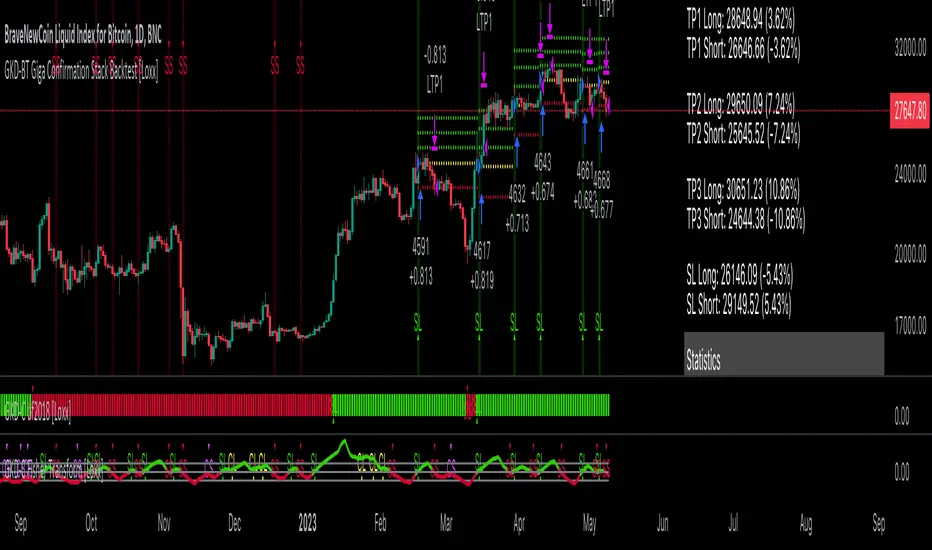
GKD-BT Giga Stacks Backtest [Loxx]Giga Kaleidoscope GKD-BT Giga Stacks Backtest is a Backtesting module included in Loxx's "Giga Kaleidoscope Modularized Trading System".
█ GKD-BT Giga Stacks Backtest
The Giga Stacks Backtest module allows users to perform backtesting on Long and Short signals from the confluence of GKD-B Baseline, GKD-C Confirmation, and GKD-V Volatility/Volume indicators. This module encompasses two types of backtests: Trading and Full. The Trading backtest permits users to evaluate individual trades, whether Long or Short, one at a time. Conversely, the Full backtest allows users to analyze either Longs or Shorts separately by toggling between them in the settings, enabling the examination of results for each signal type. The Trading backtest emulates actual trading conditions, while the Full backtest assesses all signals, regardless of being Long or Short.
Additionally, this backtest module provides the option to test using indicators with 1 to 3 take profits and 1 stop loss. The Trading backtest allows for the use of 1 to 3 take profits, while the Full backtest is limited to 1 take profit. The Trading backtest also offers the capability to apply a trailing take profit.
In terms of the percentage of trade removed at each take profit, this backtest module has the following hardcoded values:
Take profit 1: 50% of the trade is removed.
Take profit 2: 25% of the trade is removed.
Take profit 3: 25% of the trade is removed.
Stop loss: 100% of the trade is removed.
After each take profit is achieved, the stop loss level is adjusted. When take profit 1 is reached, the stop loss is moved to the entry point. Similarly, when take profit 2 is reached, the stop loss is shifted to take profit 1. The trailing take profit feature comes into play after take profit 2 or take profit 3, depending on the number of take profits selected in the settings. The trailing take profit is always activated on the final take profit when 2 or more take profits are chosen.
The backtest module also offers the capability to restrict by a specific date range, allowing for simulated forward testing based on past data. Additionally, users have the option to display or hide a trading panel that provides relevant information about the backtest, statistics, and the current trade. It is also possible to activate alerts and toggle sections of the trading panel on or off. On the chart, historical take profit and stop loss levels are represented by horizontal lines overlaid for reference.
To utilize this strategy, follow these steps (where "Stack XX" denotes the number of the Stack):
GKD-B Baseline Import: Import the value "Input into NEW GKD-BT Backtest" from the GKD-B Baseline module into the GKD-BT Giga Stacks Backtest module setting named "Stack XX: Import GKD-C, GKD-B, or GKD-V."
GKD-V Volatility/Volume Import: Import the value "Input into NEW GKD-BT Backtest" from the GKD-V Volatility/Volume module into the GKD-BT Giga Stacks Backtest module setting named "Stack XX: Import GKD-C, GKD-B, or GKD-V."
GKD-C Confirmation Import: 1) Adjust the "Confirmation Type" in the GKD-C Confirmation Indicator to "GKD New."; 2) Import the value "Input into NEW GKD-BT Backtest" from the GKD-C Confirmation module into the GKD-BT Giga Stacks Backtest module setting named "Stack XX: Import GKD-C, GKD-B, or GKD."
█ Giga Stacks Backtest Entries
Entries are generated form the confluence of up to six GKD-B Baseline, GKD-C Confirmation, and GKD-V Volatility/Volume indicators. Signals are generated when all Stacks reach uptrend or downtrend together.
Here's how this works. Assume we have the following Stacks and their respective trend on the current candle:
Stack 1 indicator is in uptreend
Stack 2 indicator is in downtrend
Stack 3 indicator is in uptreend
Stack 4 indicator is in uptreend
All stacks are in uptrend except for Stack 2. If Stack 2 reaches uptrend while Stacks 1, 3, and 4 stay in uptrend, then a long signal is generated. The last Stack to align with all other Stacks will generate a long or short signal.
█ Volatility Types Included
The GKD system utilizes volatility-based take profits and stop losses. Each take profit and stop loss is calculated as a multiple of volatility. Users can also adjust the multiplier values in the settings.
This module includes 17 types of volatility:
Close-to-Close
Parkinson
Garman-Klass
Rogers-Satchell
Yang-Zhang
Garman-Klass-Yang-Zhang
Exponential Weighted Moving Average
Standard Deviation of Log Returns
Pseudo GARCH(2,2)
Average True Range
True Range Double
Standard Deviation
Adaptive Deviation
Median Absolute Deviation
Efficiency-Ratio Adaptive ATR
Mean Absolute Deviation
Static Percent
Close-to-Close
Close-to-Close volatility is a classic and widely used volatility measure, sometimes referred to as historical volatility.
Volatility is an indicator of the speed of a stock price change. A stock with high volatility is one where the price changes rapidly and with a larger amplitude. The more volatile a stock is, the riskier it is.
Close-to-close historical volatility is calculated using only a stock's closing prices. It is the simplest volatility estimator. However, in many cases, it is not precise enough. Stock prices could jump significantly during a trading session and return to the opening value at the end. That means that a considerable amount of price information is not taken into account by close-to-close volatility.
Despite its drawbacks, Close-to-Close volatility is still useful in cases where the instrument doesn't have intraday prices. For example, mutual funds calculate their net asset values daily or weekly, and thus their prices are not suitable for more sophisticated volatility estimators.
Parkinson
Parkinson volatility is a volatility measure that uses the stock’s high and low price of the day.
The main difference between regular volatility and Parkinson volatility is that the latter uses high and low prices for a day, rather than only the closing price. This is useful as close-to-close prices could show little difference while large price movements could have occurred during the day. Thus, Parkinson's volatility is considered more precise and requires less data for calculation than close-to-close volatility.
One drawback of this estimator is that it doesn't take into account price movements after the market closes. Hence, it systematically undervalues volatility. This drawback is addressed in the Garman-Klass volatility estimator.
Garman-Klass
Garman-Klass is a volatility estimator that incorporates open, low, high, and close prices of a security.
Garman-Klass volatility extends Parkinson's volatility by taking into account the opening and closing prices. As markets are most active during the opening and closing of a trading session, it makes volatility estimation more accurate.
Garman and Klass also assumed that the process of price change follows a continuous diffusion process (Geometric Brownian motion). However, this assumption has several drawbacks. The method is not robust for opening jumps in price and trend movements.
Despite its drawbacks, the Garman-Klass estimator is still more effective than the basic formula since it takes into account not only the price at the beginning and end of the time interval but also intraday price extremes.
Researchers Rogers and Satchell have proposed a more efficient method for assessing historical volatility that takes into account price trends. See Rogers-Satchell Volatility for more detail.
Rogers-Satchell
Rogers-Satchell is an estimator for measuring the volatility of securities with an average return not equal to zero.
Unlike Parkinson and Garman-Klass estimators, Rogers-Satchell incorporates a drift term (mean return not equal to zero). As a result, it provides better volatility estimation when the underlying is trending.
The main disadvantage of this method is that it does not take into account price movements between trading sessions. This leads to an underestimation of volatility since price jumps periodically occur in the market precisely at the moments between sessions.
A more comprehensive estimator that also considers the gaps between sessions was developed based on the Rogers-Satchel formula in the 2000s by Yang-Zhang. See Yang Zhang Volatility for more detail.
Yang-Zhang
Yang Zhang is a historical volatility estimator that handles both opening jumps and the drift and has a minimum estimation error.
Yang-Zhang volatility can be thought of as a combination of the overnight (close-to-open volatility) and a weighted average of the Rogers-Satchell volatility and the day’s open-to-close volatility. It is considered to be 14 times more efficient than the close-to-close estimator.
Garman-Klass-Yang-Zhang
Garman-Klass-Yang-Zhang (GKYZ) volatility estimator incorporates the returns of open, high, low, and closing prices in its calculation.
GKYZ volatility estimator takes into account overnight jumps but not the trend, i.e., it assumes that the underlying asset follows a Geometric Brownian Motion (GBM) process with zero drift. Therefore, the GKYZ volatility estimator tends to overestimate the volatility when the drift is different from zero. However, for a GBM process, this estimator is eight times more efficient than the close-to-close volatility estimator.
Exponential Weighted Moving Average
The Exponentially Weighted Moving Average (EWMA) is a quantitative or statistical measure used to model or describe a time series. The EWMA is widely used in finance, with the main applications being technical analysis and volatility modeling.
The moving average is designed such that older observations are given lower weights. The weights decrease exponentially as the data point gets older – hence the name exponentially weighted.
The only decision a user of the EWMA must make is the parameter lambda. The parameter decides how important the current observation is in the calculation of the EWMA. The higher the value of lambda, the more closely the EWMA tracks the original time series.
Standard Deviation of Log Returns
This is the simplest calculation of volatility. It's the standard deviation of ln(close/close(1)).
Pseudo GARCH(2,2)
This is calculated using a short- and long-run mean of variance multiplied by ?.
?avg(var;M) + (1 ? ?) avg(var;N) = 2?var/(M+1-(M-1)L) + 2(1-?)var/(M+1-(M-1)L)
Solving for ? can be done by minimizing the mean squared error of estimation; that is, regressing L^-1var - avg(var; N) against avg(var; M) - avg(var; N) and using the resulting beta estimate as ?.
Average True Range
The average true range (ATR) is a technical analysis indicator, introduced by market technician J. Welles Wilder Jr. in his book New Concepts in Technical Trading Systems, that measures market volatility by decomposing the entire range of an asset price for that period.
The true range indicator is taken as the greatest of the following: current high less the current low; the absolute value of the current high less the previous close; and the absolute value of the current low less the previous close. The ATR is then a moving average, generally using 14 days, of the true ranges.
True Range Double
A special case of ATR that attempts to correct for volatility skew.
Standard Deviation
Standard deviation is a statistic that measures the dispersion of a dataset relative to its mean and is calculated as the square root of the variance. The standard deviation is calculated as the square root of variance by determining each data point's deviation relative to the mean. If the data points are further from the mean, there is a higher deviation within the data set; thus, the more spread out the data, the higher the standard deviation.
Adaptive Deviation
By definition, the Standard Deviation (STD, also represented by the Greek letter sigma ? or the Latin letter s) is a measure that is used to quantify the amount of variation or dispersion of a set of data values. In technical analysis, we usually use it to measure the level of current volatility.
Standard Deviation is based on Simple Moving Average calculation for mean value. This version of standard deviation uses the properties of EMA to calculate what can be called a new type of deviation, and since it is based on EMA, we can call it EMA deviation. Additionally, Perry Kaufman's efficiency ratio is used to make it adaptive (since all EMA type calculations are nearly perfect for adapting).
The difference when compared to the standard is significant--not just because of EMA usage, but the efficiency ratio makes it a "bit more logical" in very volatile market conditions.
Median Absolute Deviation
The median absolute deviation is a measure of statistical dispersion. Moreover, the MAD is a robust statistic, being more resilient to outliers in a data set than the standard deviation. In the standard deviation, the distances from the mean are squared, so large deviations are weighted more heavily, and thus outliers can heavily influence it. In the MAD, the deviations of a small number of outliers are irrelevant.
Because the MAD is a more robust estimator of scale than the sample variance or standard deviation, it works better with distributions without a mean or variance, such as the Cauchy distribution.
Efficiency-Ratio Adaptive ATR
Average True Range (ATR) is a widely used indicator for many occasions in technical analysis. It is calculated as the RMA of the true range. This version adds a "twist": it uses Perry Kaufman's Efficiency Ratio to calculate adaptive true range.
Mean Absolute Deviation
The mean absolute deviation (MAD) is a measure of variability that indicates the average distance between observations and their mean. MAD uses the original units of the data, which simplifies interpretation. Larger values signify that the data points spread out further from the average. Conversely, lower values correspond to data points bunching closer to it. The mean absolute deviation is also known as the mean deviation and average absolute deviation.
This definition of the mean absolute deviation sounds similar to the standard deviation (SD). While both measure variability, they have different calculations. In recent years, some proponents of MAD have suggested that it replace the SD as the primary measure because it is a simpler concept that better fits real life.
Static Percent
Static Percent allows the user to insert their own constant percent that will then be used to create take profits and stoploss
█ Giga Kaleidoscope Modularized Trading System
Core components of an NNFX algorithmic trading strategy
The NNFX algorithm is built on the principles of trend, momentum, and volatility. There are six core components in the NNFX trading algorithm:
1. Volatility - price volatility; e.g., Average True Range, True Range Double, Close-to-Close, etc.
2. Baseline - a moving average to identify price trend
3. Confirmation 1 - a technical indicator used to identify trends
4. Confirmation 2 - a technical indicator used to identify trends
5. Continuation - a technical indicator used to identify trends
6. Volatility/Volume - a technical indicator used to identify volatility/volume breakouts/breakdown
7. Exit - a technical indicator used to determine when a trend is exhausted
What is Volatility in the NNFX trading system?
In the NNFX (No Nonsense Forex) trading system, ATR (Average True Range) is typically used to measure the volatility of an asset. It is used as a part of the system to help determine the appropriate stop loss and take profit levels for a trade. ATR is calculated by taking the average of the true range values over a specified period.
True range is calculated as the maximum of the following values:
-Current high minus the current low
-Absolute value of the current high minus the previous close
-Absolute value of the current low minus the previous close
ATR is a dynamic indicator that changes with changes in volatility. As volatility increases, the value of ATR increases, and as volatility decreases, the value of ATR decreases. By using ATR in NNFX system, traders can adjust their stop loss and take profit levels according to the volatility of the asset being traded. This helps to ensure that the trade is given enough room to move, while also minimizing potential losses.
Other types of volatility include True Range Double (TRD), Close-to-Close, and Garman-Klass
What is a Baseline indicator?
The baseline is essentially a moving average, and is used to determine the overall direction of the market.
The baseline in the NNFX system is used to filter out trades that are not in line with the long-term trend of the market. The baseline is plotted on the chart along with other indicators, such as the Moving Average (MA), the Relative Strength Index (RSI), and the Average True Range (ATR).
Trades are only taken when the price is in the same direction as the baseline. For example, if the baseline is sloping upwards, only long trades are taken, and if the baseline is sloping downwards, only short trades are taken. This approach helps to ensure that trades are in line with the overall trend of the market, and reduces the risk of entering trades that are likely to fail.
By using a baseline in the NNFX system, traders can have a clear reference point for determining the overall trend of the market, and can make more informed trading decisions. The baseline helps to filter out noise and false signals, and ensures that trades are taken in the direction of the long-term trend.
What is a Confirmation indicator?
Confirmation indicators are technical indicators that are used to confirm the signals generated by primary indicators. Primary indicators are the core indicators used in the NNFX system, such as the Average True Range (ATR), the Moving Average (MA), and the Relative Strength Index (RSI).
The purpose of the confirmation indicators is to reduce false signals and improve the accuracy of the trading system. They are designed to confirm the signals generated by the primary indicators by providing additional information about the strength and direction of the trend.
Some examples of confirmation indicators that may be used in the NNFX system include the Bollinger Bands, the MACD (Moving Average Convergence Divergence), and the MACD Oscillator. These indicators can provide information about the volatility, momentum, and trend strength of the market, and can be used to confirm the signals generated by the primary indicators.
In the NNFX system, confirmation indicators are used in combination with primary indicators and other filters to create a trading system that is robust and reliable. By using multiple indicators to confirm trading signals, the system aims to reduce the risk of false signals and improve the overall profitability of the trades.
What is a Continuation indicator?
In the NNFX (No Nonsense Forex) trading system, a continuation indicator is a technical indicator that is used to confirm a current trend and predict that the trend is likely to continue in the same direction. A continuation indicator is typically used in conjunction with other indicators in the system, such as a baseline indicator, to provide a comprehensive trading strategy.
What is a Volatility/Volume indicator?
Volume indicators, such as the On Balance Volume (OBV), the Chaikin Money Flow (CMF), or the Volume Price Trend (VPT), are used to measure the amount of buying and selling activity in a market. They are based on the trading volume of the market, and can provide information about the strength of the trend. In the NNFX system, volume indicators are used to confirm trading signals generated by the Moving Average and the Relative Strength Index. Volatility indicators include Average Direction Index, Waddah Attar, and Volatility Ratio. In the NNFX trading system, volatility is a proxy for volume and vice versa.
By using volume indicators as confirmation tools, the NNFX trading system aims to reduce the risk of false signals and improve the overall profitability of trades. These indicators can provide additional information about the market that is not captured by the primary indicators, and can help traders to make more informed trading decisions. In addition, volume indicators can be used to identify potential changes in market trends and to confirm the strength of price movements.
What is an Exit indicator?
The exit indicator is used in conjunction with other indicators in the system, such as the Moving Average (MA), the Relative Strength Index (RSI), and the Average True Range (ATR), to provide a comprehensive trading strategy.
The exit indicator in the NNFX system can be any technical indicator that is deemed effective at identifying optimal exit points. Examples of exit indicators that are commonly used include the Parabolic SAR, the Average Directional Index (ADX), and the Chandelier Exit.
The purpose of the exit indicator is to identify when a trend is likely to reverse or when the market conditions have changed, signaling the need to exit a trade. By using an exit indicator, traders can manage their risk and prevent significant losses.
In the NNFX system, the exit indicator is used in conjunction with a stop loss and a take profit order to maximize profits and minimize losses. The stop loss order is used to limit the amount of loss that can be incurred if the trade goes against the trader, while the take profit order is used to lock in profits when the trade is moving in the trader's favor.
Overall, the use of an exit indicator in the NNFX trading system is an important component of a comprehensive trading strategy. It allows traders to manage their risk effectively and improve the profitability of their trades by exiting at the right time.
How does Loxx's GKD (Giga Kaleidoscope Modularized Trading System) implement the NNFX algorithm outlined above?
Loxx's GKD v2.0 system has five types of modules (indicators/strategies). These modules are:
1. GKD-BT - Backtesting module (Volatility, Number 1 in the NNFX algorithm)
2. GKD-B - Baseline module (Baseline and Volatility/Volume, Numbers 1 and 2 in the NNFX algorithm)
3. GKD-C - Confirmation 1/2 and Continuation module (Confirmation 1/2 and Continuation, Numbers 3, 4, and 5 in the NNFX algorithm)
4. GKD-V - Volatility/Volume module (Confirmation 1/2, Number 6 in the NNFX algorithm)
5. GKD-E - Exit module (Exit, Number 7 in the NNFX algorithm)
(additional module types will added in future releases)
Each module interacts with every module by passing data to A backtest module wherein the various components of the GKD system are combined to create a trading signal.
That is, the Baseline indicator passes its data to Volatility/Volume. The Volatility/Volume indicator passes its values to the Confirmation 1 indicator. The Confirmation 1 indicator passes its values to the Confirmation 2 indicator. The Confirmation 2 indicator passes its values to the Continuation indicator. The Continuation indicator passes its values to the Exit indicator, and finally, the Exit indicator passes its values to the Backtest strategy.
This chaining of indicators requires that each module conform to Loxx's GKD protocol, therefore allowing for the testing of every possible combination of technical indicators that make up the six components of the NNFX algorithm.
What does the application of the GKD trading system look like?
Example trading system:
Backtest: Stacks Backtest
Baseline: Hull Moving Average
Volatility/Volume: Hurst Exponent
Confirmation 1: Vorext
Confirmation 2: Coppock Curve
Continuation: Fisher Transform
Exit: Rex Oscillator
Each GKD indicator is denoted with a module identifier of either: GKD-BT, GKD-B, GKD-C, GKD-V, or GKD-E. This allows traders to understand to which module each indicator belongs and where each indicator fits into the GKD system.

GKD-BT Solo Confirmation Super Complex Backtest [Loxx]Giga Kaleidoscope GKD-BT Solo Confirmation Super Complex Backtest is a Backtesting module included in Loxx's "Giga Kaleidoscope Modularized Trading System".
█ GKD-BT Solo Confirmation Super Complex Backtest
The Solo Confirmation Super Complex Backtest module allows users to perform backtesting on Full GKD Long and Short signals using GKD-C confirmation indicators. These signals are further refined by GKD-B Baseline and GKD-V Volatility/Volume indicators and augmented by an additional GKD-C Confirmation indicator acting as a Continuation indicator. This module serves as a comprehensive tool that falls just below a Full GKD trading system. The key difference is that the GKD-BT Solo Confirmation Super Complex utilizes a single GKD-C Confirmation indicator, while the Full GKD system employs two GKD-C Confirmation indicators. Both the Solo Confirmation Super Complex and the Full GKD systems incorporate an extra GKD-C Confirmation indicator to identify Continuation signals, which provide both longs and shorts on developing trends following an initial trend change.
This module encompasses two types of backtests: Trading and Full. The Trading backtest permits users to evaluate individual trades, whether Long or Short, one at a time. Conversely, the Full backtest allows users to analyze either Longs or Shorts separately by toggling between them in the settings, enabling the examination of results for each signal type. The Trading backtest emulates actual trading conditions, while the Full backtest assesses all signals, regardless of being Long or Short.
Additionally, this backtest module provides the option to test the core GKD-C Confirmation and GKD-C Continuation indicators with 1 to 3 take profits and 1 stop loss. The Trading backtest allows for the use of 1 to 3 take profits, while the Full backtest is limited to 1 take profit. The Trading backtest also offers the capability to apply a trailing take profit.
In terms of the percentage of trade removed at each take profit, this backtest module has the following hardcoded values:
Take profit 1: 50% of the trade is removed.
Take profit 2: 25% of the trade is removed.
Take profit 3: 25% of the trade is removed.
Stop loss: 100% of the trade is removed.
After each take profit is achieved, the stop loss level is adjusted. When take profit 1 is reached, the stop loss is moved to the entry point. Similarly, when take profit 2 is reached, the stop loss is shifted to take profit 1. The trailing take profit feature comes into play after take profit 2 or take profit 3, depending on the number of take profits selected in the settings. The trailing take profit is always activated on the final take profit when 2 or more take profits are chosen.
The backtest module also offers the capability to restrict by a specific date range, allowing for simulated forward testing based on past data. Additionally, users have the option to display or hide a trading panel that provides relevant information about the backtest, statistics, and the current trade. It is also possible to activate alerts and toggle sections of the trading panel on or off. On the chart, historical take profit and stop loss levels are represented by horizontal lines overlaid for reference.
To utilize this strategy, follow these steps:
1. GKD-B Baseline Import: Import the value "Input into NEW GKD-BT Backtest" from the GKD-B Baseline module into the GKD-BT Solo Confirmation Super Complex Backtest module setting named "Import GKD-B Baseline."
2. GKD-V Volatility/Volume Import: Import the value "Input into NEW GKD-BT Backtest" from the GKD-V Volatility/Volume module into the GKD-BT Solo Confirmation Super Complex Backtest module setting named "Import GKD-V Volatility/Volume."
3. Adjust the "Confirmation Type" in the GKD-C Confirmation Indicator to "GKD New."
4. GKD-C Confirmation Import: Import the value "Input into NEW GKD-BT Backtest" from the GKD-C Confirmation module into the GKD-BT Solo Confirmation Super Complex Backtest module setting named "Import GKD-C Confirmation."
5. Adjust the "Confirmation Type" in the GKD-C Continuation Indicator to "GKD New."
6. GKD-C Continuation Import: Import the value "Input into NEW GKD-BT Backtest" from the GKD-C Continuation module into the GKD-BT Solo Confirmation Super Complex Backtest module setting named "Import GKD-C Continuation."
The GKD system utilizes volatility-based take profits and stop losses. Each take profit and stop loss is calculated as a multiple of volatility. Users can also adjust the multiplier values in the settings.
In a future update, the option to include a GKD-E Exit indicator will be added to this module to complete a full trading strategy.
█ Solo Confirmation Super Complex Backtest Entries
Within this module, there are eight distinct types of entries available, which are outlined below:
Standard Entry
1-Candle Standard Entry
Baseline Entry
1-Candle Baseline Entry
Volatility/Volume Entry
1-Candle Volatility/Volume Entry
PullBack Entry
Continuation Entry
Each of these entry types can generate either long or short signals, resulting in a total of 16 signal variations. The user has the flexibility to enable or disable specific entry types and choose which qualifying rules within each entry type are applied to price to determine the final long or short signal. You'll notice that these signals are different form the core GKD signals mentioned towards the end of this description. Signals from the GKD-BT Solo Confirmation Super Complex Backtest are modifided to add additional qualifications to make your finalized trading strategy more dynamic and robust.
The following section provides an overview of the various entry types and their corresponding qualifying rules:
Standard Entry
1. GKD-C Confirmation gives signal
2. Baseline agrees
3. Price inside Goldie Locks Zone Minimum
4. Price inside Goldie Locks Zone Maximum
5. Volatility/Volume agrees
1-Candle Standard Entry
1a. GKD-C Confirmation gives signal
2a. Baseline agrees
3a. Price inside Goldie Locks Zone Minimum
4a. Price inside Goldie Locks Zone Maximum
Next Candle:
1b. Price retraced
2b. Baseline agrees
3b. Confirmation 1 agrees
4b. Volatility/Volume agrees
Baseline Entry
1. GKD-B Basline gives signal
2. Confirmation 1 agrees
3. Price inside Goldie Locks Zone Minimum
4. Price inside Goldie Locks Zone Maximum
5. Volatility/Volume agrees
6. Confirmation 1 signal was less than 'Maximum Allowable PSBC Bars Back' prior
1-Candle Baseline Entry
1a. GKD-B Basline gives signal
2a. Confirmation 1 agrees
3a. Price inside Goldie Locks Zone Minimum
4a. Price inside Goldie Locks Zone Maximum
5a. Confirmation 1 signal was less than 'Maximum Allowable PSBC Bars Back' prior
Next Candle:
1b. Price retraced
2b. Baseline agrees
3b. Confirmation 1 agrees
4b. Volatility/Volume agrees
Volatility/Volume Entry
1. GKD-V Volatility/Volume gives signal
2. Confirmation 1 agrees
3. Price inside Goldie Locks Zone Minimum
4. Price inside Goldie Locks Zone Maximum
5. Baseline agrees
6. Confirmation 1 signal was less than 7 candles prior
1-Candle Volatility/Volume Entry
1a. GKD-V Volatility/Volume gives signal
2a. Confirmation 1 agrees
3a. Price inside Goldie Locks Zone Minimum
4a. Price inside Goldie Locks Zone Maximum
5a. Confirmation 1 signal was less than 'Maximum Allowable PSVVC Bars Back' prior
Next Candle:
1b. Price retraced
2b. Volatility/Volume agrees
3b. Confirmation 1 agrees
4b. Baseline agrees
PullBack Entry
1a. GKD-B Baseline gives signal
2a. Confirmation 1 agrees
3a. Price is beyond 1.0x Volatility of Baseline
Next Candle:
1b. Price inside Goldie Locks Zone Minimum
2b. Price inside Goldie Locks Zone Maximum
3b. Confirmation 1 agrees
4b. Volatility/Volume agrees
Continuation Entry
1. Standard Entry, 1-Candle Standard Entry, Baseline Entry, 1-Candle Baseline Entry, Volatility/Volume Entry, 1-Candle Volatility/Volume Entry, or Pullback entry triggered previously
2. Baseline hasn't crossed since entry signal trigger
4. Confirmation 1 agrees
5. Baseline agrees
█ Volatility Types Included
This module includes 17 types of volatility:
Close-to-Close
Parkinson
Garman-Klass
Rogers-Satchell
Yang-Zhang
Garman-Klass-Yang-Zhang
Exponential Weighted Moving Average
Standard Deviation of Log Returns
Pseudo GARCH(2,2)
Average True Range
True Range Double
Standard Deviation
Adaptive Deviation
Median Absolute Deviation
Efficiency-Ratio Adaptive ATR
Mean Absolute Deviation
Static Percent
Close-to-Close
Close-to-Close volatility is a classic and widely used volatility measure, sometimes referred to as historical volatility.
Volatility is an indicator of the speed of a stock price change. A stock with high volatility is one where the price changes rapidly and with a larger amplitude. The more volatile a stock is, the riskier it is.
Close-to-close historical volatility is calculated using only a stock's closing prices. It is the simplest volatility estimator. However, in many cases, it is not precise enough. Stock prices could jump significantly during a trading session and return to the opening value at the end. That means that a considerable amount of price information is not taken into account by close-to-close volatility.
Despite its drawbacks, Close-to-Close volatility is still useful in cases where the instrument doesn't have intraday prices. For example, mutual funds calculate their net asset values daily or weekly, and thus their prices are not suitable for more sophisticated volatility estimators.
Parkinson
Parkinson volatility is a volatility measure that uses the stock’s high and low price of the day.
The main difference between regular volatility and Parkinson volatility is that the latter uses high and low prices for a day, rather than only the closing price. This is useful as close-to-close prices could show little difference while large price movements could have occurred during the day. Thus, Parkinson's volatility is considered more precise and requires less data for calculation than close-to-close volatility.
One drawback of this estimator is that it doesn't take into account price movements after the market closes. Hence, it systematically undervalues volatility. This drawback is addressed in the Garman-Klass volatility estimator.
Garman-Klass
Garman-Klass is a volatility estimator that incorporates open, low, high, and close prices of a security.
Garman-Klass volatility extends Parkinson's volatility by taking into account the opening and closing prices. As markets are most active during the opening and closing of a trading session, it makes volatility estimation more accurate.
Garman and Klass also assumed that the process of price change follows a continuous diffusion process (Geometric Brownian motion). However, this assumption has several drawbacks. The method is not robust for opening jumps in price and trend movements.
Despite its drawbacks, the Garman-Klass estimator is still more effective than the basic formula since it takes into account not only the price at the beginning and end of the time interval but also intraday price extremes.
Researchers Rogers and Satchell have proposed a more efficient method for assessing historical volatility that takes into account price trends. See Rogers-Satchell Volatility for more detail.
Rogers-Satchell
Rogers-Satchell is an estimator for measuring the volatility of securities with an average return not equal to zero.
Unlike Parkinson and Garman-Klass estimators, Rogers-Satchell incorporates a drift term (mean return not equal to zero). As a result, it provides better volatility estimation when the underlying is trending.
The main disadvantage of this method is that it does not take into account price movements between trading sessions. This leads to an underestimation of volatility since price jumps periodically occur in the market precisely at the moments between sessions.
A more comprehensive estimator that also considers the gaps between sessions was developed based on the Rogers-Satchel formula in the 2000s by Yang-Zhang. See Yang Zhang Volatility for more detail.
Yang-Zhang
Yang Zhang is a historical volatility estimator that handles both opening jumps and the drift and has a minimum estimation error.
Yang-Zhang volatility can be thought of as a combination of the overnight (close-to-open volatility) and a weighted average of the Rogers-Satchell volatility and the day’s open-to-close volatility. It is considered to be 14 times more efficient than the close-to-close estimator.
Garman-Klass-Yang-Zhang
Garman-Klass-Yang-Zhang (GKYZ) volatility estimator incorporates the returns of open, high, low, and closing prices in its calculation.
GKYZ volatility estimator takes into account overnight jumps but not the trend, i.e., it assumes that the underlying asset follows a Geometric Brownian Motion (GBM) process with zero drift. Therefore, the GKYZ volatility estimator tends to overestimate the volatility when the drift is different from zero. However, for a GBM process, this estimator is eight times more efficient than the close-to-close volatility estimator.
Exponential Weighted Moving Average
The Exponentially Weighted Moving Average (EWMA) is a quantitative or statistical measure used to model or describe a time series. The EWMA is widely used in finance, with the main applications being technical analysis and volatility modeling.
The moving average is designed such that older observations are given lower weights. The weights decrease exponentially as the data point gets older – hence the name exponentially weighted.
The only decision a user of the EWMA must make is the parameter lambda. The parameter decides how important the current observation is in the calculation of the EWMA. The higher the value of lambda, the more closely the EWMA tracks the original time series.
Standard Deviation of Log Returns
This is the simplest calculation of volatility. It's the standard deviation of ln(close/close(1)).
Pseudo GARCH(2,2)
This is calculated using a short- and long-run mean of variance multiplied by ?.
?avg(var;M) + (1 ? ?) avg(var;N) = 2?var/(M+1-(M-1)L) + 2(1-?)var/(M+1-(M-1)L)
Solving for ? can be done by minimizing the mean squared error of estimation; that is, regressing L^-1var - avg(var; N) against avg(var; M) - avg(var; N) and using the resulting beta estimate as ?.
Average True Range
The average true range (ATR) is a technical analysis indicator, introduced by market technician J. Welles Wilder Jr. in his book New Concepts in Technical Trading Systems, that measures market volatility by decomposing the entire range of an asset price for that period.
The true range indicator is taken as the greatest of the following: current high less the current low; the absolute value of the current high less the previous close; and the absolute value of the current low less the previous close. The ATR is then a moving average, generally using 14 days, of the true ranges.
True Range Double
A special case of ATR that attempts to correct for volatility skew.
Standard Deviation
Standard deviation is a statistic that measures the dispersion of a dataset relative to its mean and is calculated as the square root of the variance. The standard deviation is calculated as the square root of variance by determining each data point's deviation relative to the mean. If the data points are further from the mean, there is a higher deviation within the data set; thus, the more spread out the data, the higher the standard deviation.
Adaptive Deviation
By definition, the Standard Deviation (STD, also represented by the Greek letter sigma ? or the Latin letter s) is a measure that is used to quantify the amount of variation or dispersion of a set of data values. In technical analysis, we usually use it to measure the level of current volatility.
Standard Deviation is based on Simple Moving Average calculation for mean value. This version of standard deviation uses the properties of EMA to calculate what can be called a new type of deviation, and since it is based on EMA, we can call it EMA deviation. Additionally, Perry Kaufman's efficiency ratio is used to make it adaptive (since all EMA type calculations are nearly perfect for adapting).
The difference when compared to the standard is significant--not just because of EMA usage, but the efficiency ratio makes it a "bit more logical" in very volatile market conditions.
Median Absolute Deviation
The median absolute deviation is a measure of statistical dispersion. Moreover, the MAD is a robust statistic, being more resilient to outliers in a data set than the standard deviation. In the standard deviation, the distances from the mean are squared, so large deviations are weighted more heavily, and thus outliers can heavily influence it. In the MAD, the deviations of a small number of outliers are irrelevant.
Because the MAD is a more robust estimator of scale than the sample variance or standard deviation, it works better with distributions without a mean or variance, such as the Cauchy distribution.
Efficiency-Ratio Adaptive ATR
Average True Range (ATR) is a widely used indicator for many occasions in technical analysis. It is calculated as the RMA of the true range. This version adds a "twist": it uses Perry Kaufman's Efficiency Ratio to calculate adaptive true range.
Mean Absolute Deviation
The mean absolute deviation (MAD) is a measure of variability that indicates the average distance between observations and their mean. MAD uses the original units of the data, which simplifies interpretation. Larger values signify that the data points spread out further from the average. Conversely, lower values correspond to data points bunching closer to it. The mean absolute deviation is also known as the mean deviation and average absolute deviation.
This definition of the mean absolute deviation sounds similar to the standard deviation (SD). While both measure variability, they have different calculations. In recent years, some proponents of MAD have suggested that it replace the SD as the primary measure because it is a simpler concept that better fits real life.
Static Percent
Static Percent allows the user to insert their own constant percent that will then be used to create take profits and stoploss
█ Giga Kaleidoscope Modularized Trading System
Core components of an NNFX algorithmic trading strategy
The NNFX algorithm is built on the principles of trend, momentum, and volatility. There are six core components in the NNFX trading algorithm:
1. Volatility - price volatility; e.g., Average True Range, True Range Double, Close-to-Close, etc.
2. Baseline - a moving average to identify price trend
3. Confirmation 1 - a technical indicator used to identify trends
4. Confirmation 2 - a technical indicator used to identify trends
5. Continuation - a technical indicator used to identify trends
6. Volatility/Volume - a technical indicator used to identify volatility/volume breakouts/breakdown
7. Exit - a technical indicator used to determine when a trend is exhausted
What is Volatility in the NNFX trading system?
In the NNFX (No Nonsense Forex) trading system, ATR (Average True Range) is typically used to measure the volatility of an asset. It is used as a part of the system to help determine the appropriate stop loss and take profit levels for a trade. ATR is calculated by taking the average of the true range values over a specified period.
True range is calculated as the maximum of the following values:
-Current high minus the current low
-Absolute value of the current high minus the previous close
-Absolute value of the current low minus the previous close
ATR is a dynamic indicator that changes with changes in volatility. As volatility increases, the value of ATR increases, and as volatility decreases, the value of ATR decreases. By using ATR in NNFX system, traders can adjust their stop loss and take profit levels according to the volatility of the asset being traded. This helps to ensure that the trade is given enough room to move, while also minimizing potential losses.
Other types of volatility include True Range Double (TRD), Close-to-Close, and Garman-Klass
What is a Baseline indicator?
The baseline is essentially a moving average, and is used to determine the overall direction of the market.
The baseline in the NNFX system is used to filter out trades that are not in line with the long-term trend of the market. The baseline is plotted on the chart along with other indicators, such as the Moving Average (MA), the Relative Strength Index (RSI), and the Average True Range (ATR).
Trades are only taken when the price is in the same direction as the baseline. For example, if the baseline is sloping upwards, only long trades are taken, and if the baseline is sloping downwards, only short trades are taken. This approach helps to ensure that trades are in line with the overall trend of the market, and reduces the risk of entering trades that are likely to fail.
By using a baseline in the NNFX system, traders can have a clear reference point for determining the overall trend of the market, and can make more informed trading decisions. The baseline helps to filter out noise and false signals, and ensures that trades are taken in the direction of the long-term trend.
What is a Confirmation indicator?
Confirmation indicators are technical indicators that are used to confirm the signals generated by primary indicators. Primary indicators are the core indicators used in the NNFX system, such as the Average True Range (ATR), the Moving Average (MA), and the Relative Strength Index (RSI).
The purpose of the confirmation indicators is to reduce false signals and improve the accuracy of the trading system. They are designed to confirm the signals generated by the primary indicators by providing additional information about the strength and direction of the trend.
Some examples of confirmation indicators that may be used in the NNFX system include the Bollinger Bands, the MACD (Moving Average Convergence Divergence), and the MACD Oscillator. These indicators can provide information about the volatility, momentum, and trend strength of the market, and can be used to confirm the signals generated by the primary indicators.
In the NNFX system, confirmation indicators are used in combination with primary indicators and other filters to create a trading system that is robust and reliable. By using multiple indicators to confirm trading signals, the system aims to reduce the risk of false signals and improve the overall profitability of the trades.
What is a Continuation indicator?
In the NNFX (No Nonsense Forex) trading system, a continuation indicator is a technical indicator that is used to confirm a current trend and predict that the trend is likely to continue in the same direction. A continuation indicator is typically used in conjunction with other indicators in the system, such as a baseline indicator, to provide a comprehensive trading strategy.
What is a Volatility/Volume indicator?
Volume indicators, such as the On Balance Volume (OBV), the Chaikin Money Flow (CMF), or the Volume Price Trend (VPT), are used to measure the amount of buying and selling activity in a market. They are based on the trading volume of the market, and can provide information about the strength of the trend. In the NNFX system, volume indicators are used to confirm trading signals generated by the Moving Average and the Relative Strength Index. Volatility indicators include Average Direction Index, Waddah Attar, and Volatility Ratio. In the NNFX trading system, volatility is a proxy for volume and vice versa.
By using volume indicators as confirmation tools, the NNFX trading system aims to reduce the risk of false signals and improve the overall profitability of trades. These indicators can provide additional information about the market that is not captured by the primary indicators, and can help traders to make more informed trading decisions. In addition, volume indicators can be used to identify potential changes in market trends and to confirm the strength of price movements.
What is an Exit indicator?
The exit indicator is used in conjunction with other indicators in the system, such as the Moving Average (MA), the Relative Strength Index (RSI), and the Average True Range (ATR), to provide a comprehensive trading strategy.
The exit indicator in the NNFX system can be any technical indicator that is deemed effective at identifying optimal exit points. Examples of exit indicators that are commonly used include the Parabolic SAR, the Average Directional Index (ADX), and the Chandelier Exit.
The purpose of the exit indicator is to identify when a trend is likely to reverse or when the market conditions have changed, signaling the need to exit a trade. By using an exit indicator, traders can manage their risk and prevent significant losses.
In the NNFX system, the exit indicator is used in conjunction with a stop loss and a take profit order to maximize profits and minimize losses. The stop loss order is used to limit the amount of loss that can be incurred if the trade goes against the trader, while the take profit order is used to lock in profits when the trade is moving in the trader's favor.
Overall, the use of an exit indicator in the NNFX trading system is an important component of a comprehensive trading strategy. It allows traders to manage their risk effectively and improve the profitability of their trades by exiting at the right time.
How does Loxx's GKD (Giga Kaleidoscope Modularized Trading System) implement the NNFX algorithm outlined above?
Loxx's GKD v2.0 system has five types of modules (indicators/strategies). These modules are:
1. GKD-BT - Backtesting module (Volatility, Number 1 in the NNFX algorithm)
2. GKD-B - Baseline module (Baseline and Volatility/Volume, Numbers 1 and 2 in the NNFX algorithm)
3. GKD-C - Confirmation 1/2 and Continuation module (Confirmation 1/2 and Continuation, Numbers 3, 4, and 5 in the NNFX algorithm)
4. GKD-V - Volatility/Volume module (Confirmation 1/2, Number 6 in the NNFX algorithm)
5. GKD-E - Exit module (Exit, Number 7 in the NNFX algorithm)
(additional module types will added in future releases)
Each module interacts with every module by passing data to A backtest module wherein the various components of the GKD system are combined to create a trading signal.
That is, the Baseline indicator passes its data to Volatility/Volume. The Volatility/Volume indicator passes its values to the Confirmation 1 indicator. The Confirmation 1 indicator passes its values to the Confirmation 2 indicator. The Confirmation 2 indicator passes its values to the Continuation indicator. The Continuation indicator passes its values to the Exit indicator, and finally, the Exit indicator passes its values to the Backtest strategy.
This chaining of indicators requires that each module conform to Loxx's GKD protocol, therefore allowing for the testing of every possible combination of technical indicators that make up the six components of the NNFX algorithm.
What does the application of the GKD trading system look like?
Example trading system:
Backtest: Solo Confirmation Complex Backtest as shown on the chart above
Baseline: Hull Moving Average as shown on the chart above
Volatility/Volume: Hurst Exponent as shown on the chart above
Confirmation 1: Fisher Trasnform as shown on the chart above
Confirmation 2: Williams Percent Range
Continuation: Vortex as shown on the chart above
Exit: Rex Oscillator
Each GKD indicator is denoted with a module identifier of either: GKD-BT, GKD-B, GKD-C, GKD-V, or GKD-E. This allows traders to understand to which module each indicator belongs and where each indicator fits into the GKD system.
Giga Kaleidoscope Modularized Trading System Signals (based on the NNFX algorithm)
Standard Entry
1. GKD-C Confirmation 1 Signal
2. GKD-B Baseline agrees
3. Price is within a range of 0.2x Volatility and 1.0x Volatility of the Goldie Locks Mean
4. GKD-C Confirmation 2 agrees
5. GKD-V Volatility/Volume agrees
Baseline Entry
1. GKD-B Baseline signal
2. GKD-C Confirmation 1 agrees
3. Price is within a range of 0.2x Volatility and 1.0x Volatility of the Goldie Locks Mean
4. GKD-C Confirmation 2 agrees
5. GKD-V Volatility/Volume agrees
6. GKD-C Confirmation 1 signal was less than 7 candles prior
Volatility/Volume Entry
1. GKD-V Volatility/Volume signal
2. GKD-C Confirmation 1 agrees
3. Price is within a range of 0.2x Volatility and 1.0x Volatility of the Goldie Locks Mean
4. GKD-C Confirmation 2 agrees
5. GKD-B Baseline agrees
6. GKD-C Confirmation 1 signal was less than 7 candles prior
Continuation Entry
1. Standard Entry, Baseline Entry, or Pullback; entry triggered previously
2. GKD-B Baseline hasn't crossed since entry signal trigger
3. GKD-C Confirmation Continuation Indicator signals
4. GKD-C Confirmation 1 agrees
5. GKD-B Baseline agrees
6. GKD-C Confirmation 2 agrees
1-Candle Rule Standard Entry
1. GKD-C Confirmation 1 signal
2. GKD-B Baseline agrees
3. Price is within a range of 0.2x Volatility and 1.0x Volatility of the Goldie Locks Mean
Next Candle:
1. Price retraced (Long: close < close or Short: close > close )
2. GKD-B Baseline agrees
3. GKD-C Confirmation 1 agrees
4. GKD-C Confirmation 2 agrees
5. GKD-V Volatility/Volume agrees
1-Candle Rule Baseline Entry
1. GKD-B Baseline signal
2. GKD-C Confirmation 1 agrees
3. Price is within a range of 0.2x Volatility and 1.0x Volatility of the Goldie Locks Mean
4. GKD-C Confirmation 1 signal was less than 7 candles prior
Next Candle:
1. Price retraced (Long: close < close or Short: close > close )
2. GKD-B Baseline agrees
3. GKD-C Confirmation 1 agrees
4. GKD-C Confirmation 2 agrees
5. GKD-V Volatility/Volume Agrees
1-Candle Rule Volatility/Volume Entry
1. GKD-V Volatility/Volume signal
2. GKD-C Confirmation 1 agrees
3. Price is within a range of 0.2x Volatility and 1.0x Volatility of the Goldie Locks Mean
4. GKD-C Confirmation 1 signal was less than 7 candles prior
Next Candle:
1. Price retraced (Long: close < close or Short: close > close)
2. GKD-B Volatility/Volume agrees
3. GKD-C Confirmation 1 agrees
4. GKD-C Confirmation 2 agrees
5. GKD-B Baseline agrees
PullBack Entry
1. GKD-B Baseline signal
2. GKD-C Confirmation 1 agrees
3. Price is beyond 1.0x Volatility of Baseline
Next Candle:
1. Price is within a range of 0.2x Volatility and 1.0x Volatility of the Goldie Locks Mean
2. GKD-C Confirmation 1 agrees
3. GKD-C Confirmation 2 agrees
4. GKD-V Volatility/Volume Agrees

GKD-BT Solo Confirmation Complex Backtest [Loxx]Giga Kaleidoscope GKD-BT Solo Confirmation Complex Backtest is a Backtesting module included in Loxx's "Giga Kaleidoscope Modularized Trading System".
█ GKD-BT Solo Confirmation Complex Backtest
The Solo Confirmation Complex Backtest module enables users to perform backtesting on Standard Long and Short signals from GKD-C confirmation indicators, filtered by GKD-B Baseline and GKD-V Volatility/Volume indicators. This module represents a complex form of the Solo Confirmation Backtest in the GKD trading system. It includes two types of backtests: Trading and Full. The Trading backtest allows users to test individual trades, both Long and Short, one at a time. On the other hand, the Full backtest allows users to test either Longs or Shorts by toggling between them in the settings to view the results for each signal type. The Trading backtest simulates real trading, while the Full backtest tests all signals, whether Long or Short.
Additionally, this backtest module provides the option to test the GKD-C Confirmation indicator with 1 to 3 take profits and 1 stop loss. The Trading backtest allows for the use of 1 to 3 take profits, while the Full backtest is limited to 1 take profit. The Trading backtest also offers the capability to apply a trailing take profit.
In terms of the percentage of trade removed at each take profit, this backtest module has the following hardcoded values:
Take profit 1: 50% of the trade is removed.
Take profit 2: 25% of the trade is removed.
Take profit 3: 25% of the trade is removed.
Stop loss: 100% of the trade is removed.
After each take profit is achieved, the stop loss level is adjusted. When take profit 1 is reached, the stop loss is moved to the entry point. Similarly, when take profit 2 is reached, the stop loss is shifted to take profit 1. The trailing take profit feature comes into play after take profit 2 or take profit 3, depending on the number of take profits selected in the settings. The trailing take profit is always activated on the final take profit when 2 or more take profits are chosen.
The backtest module also offers the capability to restrict by a specific date range, allowing for simulated forward testing based on past data. Additionally, users have the option to display or hide a trading panel that provides relevant information about the backtest, statistics, and the current trade. It is also possible to activate alerts and toggle sections of the trading panel on or off. On the chart, historical take profit and stop loss levels are represented by horizontal lines overlaid for reference.
The GKD system utilizes volatility-based take profits and stop losses. Each take profit and stop loss is calculated as a multiple of volatility. Users can also adjust the multiplier values in the settings.
To utilize this strategy, follow these steps:
1. GKD-B Baseline Import: Import the value "Input into NEW GKD-BT Backtest" from the GKD-B Baseline module into the GKD-BT Solo Confirmation Complex Backtest module setting named "Import GKD-B Baseline indicator."
Adjust the "Confirmation Type" in the GKD-C Confirmation Indicator to "GKD New."
2. GKD-C Confirmation Import: Import the value "Input into NEW GKD-BT Backtest" from the GKD-C Confirmation module into the GKD-BT Solo Confirmation Complex Backtest module setting named "Import GKD-C Confirmation indicator."
3. GKD-V Volatility/Volume Import: Import the value "Input into NEW GKD-BT Backtest" from the GKD-V Volatility/Volume module into the GKD-BT Solo Confirmation Complex Backtest module setting named "Import GKD-V Volatility/Volume indicator."
4. The Solo Confirmation Complex Backtest module exclusively supports Standard Entries, both Long and Short. However, please note that this module uses a modified version of the Standard Entry. In this modified version, long and short signals are directly imported from the Confirmation indicator, and then baseline and volatility filtering is applied.
The GKD-B Baseline filter ensures that only trades aligning with the GKD-B Baseline's current trend are accepted. This filter takes into consideration the Goldie Locks Zone, which allows trades where the closing price of the last candle has moved within a minimum XX volatility and a maximum YY volatility range. The GKD-V Volatility/Volume filter allows only trades that meet a minimum threshold of ZZ GKD-V Volatility/Volume, which varies based on the specific GKD-V Volatility/Volume indicator used.
The Solo Confirmation Complex Backtest execution engine determines whether signals from the GKD-C Confirmation indicator are accepted or rejected based on two criteria:
1. The GKD-C Confirmation signal must be qualified by the direction of the GKD-B Baseline trend and the GKD-B Baseline's sweet-spot Goldie Locks Zone.
2. Sufficient Volatility/Volume, as indicated by the GKD-V Volatility/Volume indicator, must be present to execute a trade.
The purpose of the Solo Confirmation Complex Backtest is to test a GKD-C Confirmation indicator in the presence of macro trend and volatility/volume filtering.
Volatility Types Included
17 types of volatility are included in this indicator
Close-to-Close
Parkinson
Garman-Klass
Rogers-Satchell
Yang-Zhang
Garman-Klass-Yang-Zhang
Exponential Weighted Moving Average
Standard Deviation of Log Returns
Pseudo GARCH(2,2)
Average True Range
True Range Double
Standard Deviation
Adaptive Deviation
Median Absolute Deviation
Efficiency-Ratio Adaptive ATR
Mean Absolute Deviation
Static Percent
Close-to-Close
Close-to-Close volatility is a classic and widely used volatility measure, sometimes referred to as historical volatility.
Volatility is an indicator of the speed of a stock price change. A stock with high volatility is one where the price changes rapidly and with a larger amplitude. The more volatile a stock is, the riskier it is.
Close-to-close historical volatility is calculated using only a stock's closing prices. It is the simplest volatility estimator. However, in many cases, it is not precise enough. Stock prices could jump significantly during a trading session and return to the opening value at the end. That means that a considerable amount of price information is not taken into account by close-to-close volatility.
Despite its drawbacks, Close-to-Close volatility is still useful in cases where the instrument doesn't have intraday prices. For example, mutual funds calculate their net asset values daily or weekly, and thus their prices are not suitable for more sophisticated volatility estimators.
Parkinson
Parkinson volatility is a volatility measure that uses the stock’s high and low price of the day.
The main difference between regular volatility and Parkinson volatility is that the latter uses high and low prices for a day, rather than only the closing price. This is useful as close-to-close prices could show little difference while large price movements could have occurred during the day. Thus, Parkinson's volatility is considered more precise and requires less data for calculation than close-to-close volatility.
One drawback of this estimator is that it doesn't take into account price movements after the market closes. Hence, it systematically undervalues volatility. This drawback is addressed in the Garman-Klass volatility estimator.
Garman-Klass
Garman-Klass is a volatility estimator that incorporates open, low, high, and close prices of a security.
Garman-Klass volatility extends Parkinson's volatility by taking into account the opening and closing prices. As markets are most active during the opening and closing of a trading session, it makes volatility estimation more accurate.
Garman and Klass also assumed that the process of price change follows a continuous diffusion process (Geometric Brownian motion). However, this assumption has several drawbacks. The method is not robust for opening jumps in price and trend movements.
Despite its drawbacks, the Garman-Klass estimator is still more effective than the basic formula since it takes into account not only the price at the beginning and end of the time interval but also intraday price extremes.
Researchers Rogers and Satchell have proposed a more efficient method for assessing historical volatility that takes into account price trends. See Rogers-Satchell Volatility for more detail.
Rogers-Satchell
Rogers-Satchell is an estimator for measuring the volatility of securities with an average return not equal to zero.
Unlike Parkinson and Garman-Klass estimators, Rogers-Satchell incorporates a drift term (mean return not equal to zero). As a result, it provides better volatility estimation when the underlying is trending.
The main disadvantage of this method is that it does not take into account price movements between trading sessions. This leads to an underestimation of volatility since price jumps periodically occur in the market precisely at the moments between sessions.
A more comprehensive estimator that also considers the gaps between sessions was developed based on the Rogers-Satchel formula in the 2000s by Yang-Zhang. See Yang Zhang Volatility for more detail.
Yang-Zhang
Yang Zhang is a historical volatility estimator that handles both opening jumps and the drift and has a minimum estimation error.
Yang-Zhang volatility can be thought of as a combination of the overnight (close-to-open volatility) and a weighted average of the Rogers-Satchell volatility and the day’s open-to-close volatility. It is considered to be 14 times more efficient than the close-to-close estimator.
Garman-Klass-Yang-Zhang
Garman-Klass-Yang-Zhang (GKYZ) volatility estimator incorporates the returns of open, high, low, and closing prices in its calculation.
GKYZ volatility estimator takes into account overnight jumps but not the trend, i.e., it assumes that the underlying asset follows a Geometric Brownian Motion (GBM) process with zero drift. Therefore, the GKYZ volatility estimator tends to overestimate the volatility when the drift is different from zero. However, for a GBM process, this estimator is eight times more efficient than the close-to-close volatility estimator.
Exponential Weighted Moving Average
The Exponentially Weighted Moving Average (EWMA) is a quantitative or statistical measure used to model or describe a time series. The EWMA is widely used in finance, with the main applications being technical analysis and volatility modeling.
The moving average is designed such that older observations are given lower weights. The weights decrease exponentially as the data point gets older – hence the name exponentially weighted.
The only decision a user of the EWMA must make is the parameter lambda. The parameter decides how important the current observation is in the calculation of the EWMA. The higher the value of lambda, the more closely the EWMA tracks the original time series.
Standard Deviation of Log Returns
This is the simplest calculation of volatility. It's the standard deviation of ln(close/close(1)).
Pseudo GARCH(2,2)
This is calculated using a short- and long-run mean of variance multiplied by ?.
?avg(var;M) + (1 ? ?) avg(var;N) = 2?var/(M+1-(M-1)L) + 2(1-?)var/(M+1-(M-1)L)
Solving for ? can be done by minimizing the mean squared error of estimation; that is, regressing L^-1var - avg(var; N) against avg(var; M) - avg(var; N) and using the resulting beta estimate as ?.
Average True Range
The average true range (ATR) is a technical analysis indicator, introduced by market technician J. Welles Wilder Jr. in his book New Concepts in Technical Trading Systems, that measures market volatility by decomposing the entire range of an asset price for that period.
The true range indicator is taken as the greatest of the following: current high less the current low; the absolute value of the current high less the previous close; and the absolute value of the current low less the previous close. The ATR is then a moving average, generally using 14 days, of the true ranges.
True Range Double
A special case of ATR that attempts to correct for volatility skew.
Standard Deviation
Standard deviation is a statistic that measures the dispersion of a dataset relative to its mean and is calculated as the square root of the variance. The standard deviation is calculated as the square root of variance by determining each data point's deviation relative to the mean. If the data points are further from the mean, there is a higher deviation within the data set; thus, the more spread out the data, the higher the standard deviation.
Adaptive Deviation
By definition, the Standard Deviation (STD, also represented by the Greek letter sigma ? or the Latin letter s) is a measure that is used to quantify the amount of variation or dispersion of a set of data values. In technical analysis, we usually use it to measure the level of current volatility.
Standard Deviation is based on Simple Moving Average calculation for mean value. This version of standard deviation uses the properties of EMA to calculate what can be called a new type of deviation, and since it is based on EMA, we can call it EMA deviation. Additionally, Perry Kaufman's efficiency ratio is used to make it adaptive (since all EMA type calculations are nearly perfect for adapting).
The difference when compared to the standard is significant--not just because of EMA usage, but the efficiency ratio makes it a "bit more logical" in very volatile market conditions.
Median Absolute Deviation
The median absolute deviation is a measure of statistical dispersion. Moreover, the MAD is a robust statistic, being more resilient to outliers in a data set than the standard deviation. In the standard deviation, the distances from the mean are squared, so large deviations are weighted more heavily, and thus outliers can heavily influence it. In the MAD, the deviations of a small number of outliers are irrelevant.
Because the MAD is a more robust estimator of scale than the sample variance or standard deviation, it works better with distributions without a mean or variance, such as the Cauchy distribution.
Efficiency-Ratio Adaptive ATR
Average True Range (ATR) is a widely used indicator for many occasions in technical analysis. It is calculated as the RMA of the true range. This version adds a "twist": it uses Perry Kaufman's Efficiency Ratio to calculate adaptive true range.
Mean Absolute Deviation
The mean absolute deviation (MAD) is a measure of variability that indicates the average distance between observations and their mean. MAD uses the original units of the data, which simplifies interpretation. Larger values signify that the data points spread out further from the average. Conversely, lower values correspond to data points bunching closer to it. The mean absolute deviation is also known as the mean deviation and average absolute deviation.
This definition of the mean absolute deviation sounds similar to the standard deviation (SD). While both measure variability, they have different calculations. In recent years, some proponents of MAD have suggested that it replace the SD as the primary measure because it is a simpler concept that better fits real life.
Static Percent
Static Percent allows the user to insert their own constant percent that will then be used to create take profits and stoploss
█ Giga Kaleidoscope Modularized Trading System
Core components of an NNFX algorithmic trading strategy
The NNFX algorithm is built on the principles of trend, momentum, and volatility. There are six core components in the NNFX trading algorithm:
1. Volatility - price volatility; e.g., Average True Range, True Range Double, Close-to-Close, etc.
2. Baseline - a moving average to identify price trend
3. Confirmation 1 - a technical indicator used to identify trends
4. Confirmation 2 - a technical indicator used to identify trends
5. Continuation - a technical indicator used to identify trends
6. Volatility/Volume - a technical indicator used to identify volatility/volume breakouts/breakdown
7. Exit - a technical indicator used to determine when a trend is exhausted
What is Volatility in the NNFX trading system?
In the NNFX (No Nonsense Forex) trading system, ATR (Average True Range) is typically used to measure the volatility of an asset. It is used as a part of the system to help determine the appropriate stop loss and take profit levels for a trade. ATR is calculated by taking the average of the true range values over a specified period.
True range is calculated as the maximum of the following values:
-Current high minus the current low
-Absolute value of the current high minus the previous close
-Absolute value of the current low minus the previous close
ATR is a dynamic indicator that changes with changes in volatility. As volatility increases, the value of ATR increases, and as volatility decreases, the value of ATR decreases. By using ATR in NNFX system, traders can adjust their stop loss and take profit levels according to the volatility of the asset being traded. This helps to ensure that the trade is given enough room to move, while also minimizing potential losses.
Other types of volatility include True Range Double (TRD), Close-to-Close, and Garman-Klass
What is a Baseline indicator?
The baseline is essentially a moving average, and is used to determine the overall direction of the market.
The baseline in the NNFX system is used to filter out trades that are not in line with the long-term trend of the market. The baseline is plotted on the chart along with other indicators, such as the Moving Average (MA), the Relative Strength Index (RSI), and the Average True Range (ATR).
Trades are only taken when the price is in the same direction as the baseline. For example, if the baseline is sloping upwards, only long trades are taken, and if the baseline is sloping downwards, only short trades are taken. This approach helps to ensure that trades are in line with the overall trend of the market, and reduces the risk of entering trades that are likely to fail.
By using a baseline in the NNFX system, traders can have a clear reference point for determining the overall trend of the market, and can make more informed trading decisions. The baseline helps to filter out noise and false signals, and ensures that trades are taken in the direction of the long-term trend.
What is a Confirmation indicator?
Confirmation indicators are technical indicators that are used to confirm the signals generated by primary indicators. Primary indicators are the core indicators used in the NNFX system, such as the Average True Range (ATR), the Moving Average (MA), and the Relative Strength Index (RSI).
The purpose of the confirmation indicators is to reduce false signals and improve the accuracy of the trading system. They are designed to confirm the signals generated by the primary indicators by providing additional information about the strength and direction of the trend.
Some examples of confirmation indicators that may be used in the NNFX system include the Bollinger Bands, the MACD (Moving Average Convergence Divergence), and the MACD Oscillator. These indicators can provide information about the volatility, momentum, and trend strength of the market, and can be used to confirm the signals generated by the primary indicators.
In the NNFX system, confirmation indicators are used in combination with primary indicators and other filters to create a trading system that is robust and reliable. By using multiple indicators to confirm trading signals, the system aims to reduce the risk of false signals and improve the overall profitability of the trades.
What is a Continuation indicator?
In the NNFX (No Nonsense Forex) trading system, a continuation indicator is a technical indicator that is used to confirm a current trend and predict that the trend is likely to continue in the same direction. A continuation indicator is typically used in conjunction with other indicators in the system, such as a baseline indicator, to provide a comprehensive trading strategy.
What is a Volatility/Volume indicator?
Volume indicators, such as the On Balance Volume (OBV), the Chaikin Money Flow (CMF), or the Volume Price Trend (VPT), are used to measure the amount of buying and selling activity in a market. They are based on the trading volume of the market, and can provide information about the strength of the trend. In the NNFX system, volume indicators are used to confirm trading signals generated by the Moving Average and the Relative Strength Index. Volatility indicators include Average Direction Index, Waddah Attar, and Volatility Ratio. In the NNFX trading system, volatility is a proxy for volume and vice versa.
By using volume indicators as confirmation tools, the NNFX trading system aims to reduce the risk of false signals and improve the overall profitability of trades. These indicators can provide additional information about the market that is not captured by the primary indicators, and can help traders to make more informed trading decisions. In addition, volume indicators can be used to identify potential changes in market trends and to confirm the strength of price movements.
What is an Exit indicator?
The exit indicator is used in conjunction with other indicators in the system, such as the Moving Average (MA), the Relative Strength Index (RSI), and the Average True Range (ATR), to provide a comprehensive trading strategy.
The exit indicator in the NNFX system can be any technical indicator that is deemed effective at identifying optimal exit points. Examples of exit indicators that are commonly used include the Parabolic SAR, the Average Directional Index (ADX), and the Chandelier Exit.
The purpose of the exit indicator is to identify when a trend is likely to reverse or when the market conditions have changed, signaling the need to exit a trade. By using an exit indicator, traders can manage their risk and prevent significant losses.
In the NNFX system, the exit indicator is used in conjunction with a stop loss and a take profit order to maximize profits and minimize losses. The stop loss order is used to limit the amount of loss that can be incurred if the trade goes against the trader, while the take profit order is used to lock in profits when the trade is moving in the trader's favor.
Overall, the use of an exit indicator in the NNFX trading system is an important component of a comprehensive trading strategy. It allows traders to manage their risk effectively and improve the profitability of their trades by exiting at the right time.
How does Loxx's GKD (Giga Kaleidoscope Modularized Trading System) implement the NNFX algorithm outlined above?
Loxx's GKD v2.0 system has five types of modules (indicators/strategies). These modules are:
1. GKD-BT - Backtesting module (Volatility, Number 1 in the NNFX algorithm)
2. GKD-B - Baseline module (Baseline and Volatility/Volume, Numbers 1 and 2 in the NNFX algorithm)
3. GKD-C - Confirmation 1/2 and Continuation module (Confirmation 1/2 and Continuation, Numbers 3, 4, and 5 in the NNFX algorithm)
4. GKD-V - Volatility/Volume module (Confirmation 1/2, Number 6 in the NNFX algorithm)
5. GKD-E - Exit module (Exit, Number 7 in the NNFX algorithm)
(additional module types will added in future releases)
Each module interacts with every module by passing data to A backtest module wherein the various components of the GKD system are combined to create a trading signal.
That is, the Baseline indicator passes its data to Volatility/Volume. The Volatility/Volume indicator passes its values to the Confirmation 1 indicator. The Confirmation 1 indicator passes its values to the Confirmation 2 indicator. The Confirmation 2 indicator passes its values to the Continuation indicator. The Continuation indicator passes its values to the Exit indicator, and finally, the Exit indicator passes its values to the Backtest strategy.
This chaining of indicators requires that each module conform to Loxx's GKD protocol, therefore allowing for the testing of every possible combination of technical indicators that make up the six components of the NNFX algorithm.
What does the application of the GKD trading system look like?
Example trading system:
Backtest: Solo Confirmation Complex Backtest as shown on the chart above
Baseline: Hull Moving Average as shown on the chart above
Volatility/Volume: Hurst Exponent as shown on the chart above
Confirmation 1: Fisher Trasnform as shown on the chart above
Confirmation 2: Williams Percent Range
Continuation: Volatility-Adaptive Rapid RSI T3
Exit: Rex Oscillator
Each GKD indicator is denoted with a module identifier of either: GKD-BT, GKD-B, GKD-C, GKD-V, or GKD-E. This allows traders to understand to which module each indicator belongs and where each indicator fits into the GKD system.
Giga Kaleidoscope Modularized Trading System Signals (based on the NNFX algorithm)
Standard Entry
1. GKD-C Confirmation 1 Signal
2. GKD-B Baseline agrees
3. Price is within a range of 0.2x Volatility and 1.0x Volatility of the Goldie Locks Mean
4. GKD-C Confirmation 2 agrees
5. GKD-V Volatility/Volume agrees
Baseline Entry
1. GKD-B Baseline signal
2. GKD-C Confirmation 1 agrees
3. Price is within a range of 0.2x Volatility and 1.0x Volatility of the Goldie Locks Mean
4. GKD-C Confirmation 2 agrees
5. GKD-V Volatility/Volume agrees
6. GKD-C Confirmation 1 signal was less than 7 candles prior
Volatility/Volume Entry
1. GKD-V Volatility/Volume signal
2. GKD-C Confirmation 1 agrees
3. Price is within a range of 0.2x Volatility and 1.0x Volatility of the Goldie Locks Mean
4. GKD-C Confirmation 2 agrees
5. GKD-B Baseline agrees
6. GKD-C Confirmation 1 signal was less than 7 candles prior
Continuation Entry
1. Standard Entry, Baseline Entry, or Pullback; entry triggered previously
2. GKD-B Baseline hasn't crossed since entry signal trigger
3. GKD-C Confirmation Continuation Indicator signals
4. GKD-C Confirmation 1 agrees
5. GKD-B Baseline agrees
6. GKD-C Confirmation 2 agrees
1-Candle Rule Standard Entry
1. GKD-C Confirmation 1 signal
2. GKD-B Baseline agrees
3. Price is within a range of 0.2x Volatility and 1.0x Volatility of the Goldie Locks Mean
Next Candle:
1. Price retraced (Long: close < close or Short: close > close )
2. GKD-B Baseline agrees
3. GKD-C Confirmation 1 agrees
4. GKD-C Confirmation 2 agrees
5. GKD-V Volatility/Volume agrees
1-Candle Rule Baseline Entry
1. GKD-B Baseline signal
2. GKD-C Confirmation 1 agrees
3. Price is within a range of 0.2x Volatility and 1.0x Volatility of the Goldie Locks Mean
4. GKD-C Confirmation 1 signal was less than 7 candles prior
Next Candle:
1. Price retraced (Long: close < close or Short: close > close )
2. GKD-B Baseline agrees
3. GKD-C Confirmation 1 agrees
4. GKD-C Confirmation 2 agrees
5. GKD-V Volatility/Volume Agrees
1-Candle Rule Volatility/Volume Entry
1. GKD-V Volatility/Volume signal
2. GKD-C Confirmation 1 agrees
3. Price is within a range of 0.2x Volatility and 1.0x Volatility of the Goldie Locks Mean
4. GKD-C Confirmation 1 signal was less than 7 candles prior
Next Candle:
1. Price retraced (Long: close < close or Short: close > close)
2. GKD-B Volatility/Volume agrees
3. GKD-C Confirmation 1 agrees
4. GKD-C Confirmation 2 agrees
5. GKD-B Baseline agrees
PullBack Entry
1. GKD-B Baseline signal
2. GKD-C Confirmation 1 agrees
3. Price is beyond 1.0x Volatility of Baseline
Next Candle:
1. Price is within a range of 0.2x Volatility and 1.0x Volatility of the Goldie Locks Mean
2. GKD-C Confirmation 1 agrees
3. GKD-C Confirmation 2 agrees
4. GKD-V Volatility/Volume Agrees
GKD-BT Solo Confirmation Simple Backtest [Loxx]Giga Kaleidoscope GKD-BT Solo Confirmation Simple Backtest is a Backtesting module included in Loxx's "Giga Kaleidoscope Modularized Trading System".
█ GKD-BT Solo Confirmation Simple Backtest
The Solo Confirmation Simple Backtest module enables users to perform Standard Long and Short signals on GKD-C confirmation indicators. This module represents the simplest form of Backtest in the GKD trading system. It includes two types of backtests: Trading and Full. The Trading backtest allows users to test individual trades, both long and short, one at a time. On the other hand, the Full backtest allows users to test either longs or shorts by toggling between them in the settings to view the results for each signal type. The Trading backtest simulates real trading, while the Full backtest tests all signals, whether long or short.
Additionally, this backtest module provides the option to test the GKD-C indicator with 1 to 3 take profits and 1 stop loss. The Trading backtest allows for the use of 1 to 3 take profits, while the Full backtest is limited to 1 take profit. The Trading backtest also offers the capability to apply a trailing take profit.
In terms of the percentage of trade removed at each take profit, this backtest module has the following hardcoded values:
Take profit 1: 50% of the trade is removed
Take profit 2: 25% of the trade is removed
Take profit 3: 25% of the trade is removed
Stop loss: 100% of the trade is removed
After each take profit is achieved, the stop loss level is adjusted. When take profit 1 is reached, the stop loss is moved to the entry point. Similarly, when take profit 2 is reached, the stop loss is shifted to take profit 1. The trailing take profit feature comes into play after take profit 2 or take profit 3, depending on the number of take profits selected in the settings. The trailing take profit is always activated on the final take profit when 2 or more take profits are chosen.
The backtest also offers the capability to restrict by a specific date range, allowing for simulated forward testing based on past data. Additionally, users have the option to display or hide a trading panel that provides relevant information about the backtest, statistics, and the current trade. It is also possible to activate alerts and toggle sections of the trading panel on or off. On the chart, historical take profit and stop loss levels are represented by horizontal lines overlaid for reference.
The GKD system utilizes volatility-based take profits and stop losses. Each take profit and stop loss is calculated as a multiple of volatility. You can change the values of the multipliers in the settings as well.
To utilize this strategy, follow these steps:
1. Adjust the "Confirmation Type" in the GKD-C Confirmation Indicator to "GKD New."
2. Import the value "Input into NEW GKD-BT Backtest" into the GKD-BT Solo Confirmation Simple Backtest module (this strategy backtest).
**The GKD-BT Solo Confirmation Simple Backtest module exclusively supports Standard Entries, both Long and Short. However, please note that this module uses a modified version of the standard entry, where long and short signals are directly imported from the Confirmation indicator without any baseline or volatility filtering applied.**
Volatility Types Included
17 types of volatility are included in this indicator
Close-to-Close
Parkinson
Garman-Klass
Rogers-Satchell
Yang-Zhang
Garman-Klass-Yang-Zhang
Exponential Weighted Moving Average
Standard Deviation of Log Returns
Pseudo GARCH(2,2)
Average True Range
True Range Double
Standard Deviation
Adaptive Deviation
Median Absolute Deviation
Efficiency-Ratio Adaptive ATR
Mean Absolute Deviation
Static Percent
Close-to-Close
Close-to-Close volatility is a classic and widely used volatility measure, sometimes referred to as historical volatility.
Volatility is an indicator of the speed of a stock price change. A stock with high volatility is one where the price changes rapidly and with a larger amplitude. The more volatile a stock is, the riskier it is.
Close-to-close historical volatility is calculated using only a stock's closing prices. It is the simplest volatility estimator. However, in many cases, it is not precise enough. Stock prices could jump significantly during a trading session and return to the opening value at the end. That means that a considerable amount of price information is not taken into account by close-to-close volatility.
Despite its drawbacks, Close-to-Close volatility is still useful in cases where the instrument doesn't have intraday prices. For example, mutual funds calculate their net asset values daily or weekly, and thus their prices are not suitable for more sophisticated volatility estimators.
Parkinson
Parkinson volatility is a volatility measure that uses the stock’s high and low price of the day.
The main difference between regular volatility and Parkinson volatility is that the latter uses high and low prices for a day, rather than only the closing price. This is useful as close-to-close prices could show little difference while large price movements could have occurred during the day. Thus, Parkinson's volatility is considered more precise and requires less data for calculation than close-to-close volatility.
One drawback of this estimator is that it doesn't take into account price movements after the market closes. Hence, it systematically undervalues volatility. This drawback is addressed in the Garman-Klass volatility estimator.
Garman-Klass
Garman-Klass is a volatility estimator that incorporates open, low, high, and close prices of a security.
Garman-Klass volatility extends Parkinson's volatility by taking into account the opening and closing prices. As markets are most active during the opening and closing of a trading session, it makes volatility estimation more accurate.
Garman and Klass also assumed that the process of price change follows a continuous diffusion process (Geometric Brownian motion). However, this assumption has several drawbacks. The method is not robust for opening jumps in price and trend movements.
Despite its drawbacks, the Garman-Klass estimator is still more effective than the basic formula since it takes into account not only the price at the beginning and end of the time interval but also intraday price extremes.
Researchers Rogers and Satchell have proposed a more efficient method for assessing historical volatility that takes into account price trends. See Rogers-Satchell Volatility for more detail.
Rogers-Satchell
Rogers-Satchell is an estimator for measuring the volatility of securities with an average return not equal to zero.
Unlike Parkinson and Garman-Klass estimators, Rogers-Satchell incorporates a drift term (mean return not equal to zero). As a result, it provides better volatility estimation when the underlying is trending.
The main disadvantage of this method is that it does not take into account price movements between trading sessions. This leads to an underestimation of volatility since price jumps periodically occur in the market precisely at the moments between sessions.
A more comprehensive estimator that also considers the gaps between sessions was developed based on the Rogers-Satchel formula in the 2000s by Yang-Zhang. See Yang Zhang Volatility for more detail.
Yang-Zhang
Yang Zhang is a historical volatility estimator that handles both opening jumps and the drift and has a minimum estimation error.
Yang-Zhang volatility can be thought of as a combination of the overnight (close-to-open volatility) and a weighted average of the Rogers-Satchell volatility and the day’s open-to-close volatility. It is considered to be 14 times more efficient than the close-to-close estimator.
Garman-Klass-Yang-Zhang
Garman-Klass-Yang-Zhang (GKYZ) volatility estimator incorporates the returns of open, high, low, and closing prices in its calculation.
GKYZ volatility estimator takes into account overnight jumps but not the trend, i.e., it assumes that the underlying asset follows a Geometric Brownian Motion (GBM) process with zero drift. Therefore, the GKYZ volatility estimator tends to overestimate the volatility when the drift is different from zero. However, for a GBM process, this estimator is eight times more efficient than the close-to-close volatility estimator.
Exponential Weighted Moving Average
The Exponentially Weighted Moving Average (EWMA) is a quantitative or statistical measure used to model or describe a time series. The EWMA is widely used in finance, with the main applications being technical analysis and volatility modeling.
The moving average is designed such that older observations are given lower weights. The weights decrease exponentially as the data point gets older – hence the name exponentially weighted.
The only decision a user of the EWMA must make is the parameter lambda. The parameter decides how important the current observation is in the calculation of the EWMA. The higher the value of lambda, the more closely the EWMA tracks the original time series.
Standard Deviation of Log Returns
This is the simplest calculation of volatility. It's the standard deviation of ln(close/close(1)).
Pseudo GARCH(2,2)
This is calculated using a short- and long-run mean of variance multiplied by ?.
?avg(var;M) + (1 ? ?) avg(var;N) = 2?var/(M+1-(M-1)L) + 2(1-?)var/(M+1-(M-1)L)
Solving for ? can be done by minimizing the mean squared error of estimation; that is, regressing L^-1var - avg(var; N) against avg(var; M) - avg(var; N) and using the resulting beta estimate as ?.
Average True Range
The average true range (ATR) is a technical analysis indicator, introduced by market technician J. Welles Wilder Jr. in his book New Concepts in Technical Trading Systems, that measures market volatility by decomposing the entire range of an asset price for that period.
The true range indicator is taken as the greatest of the following: current high less the current low; the absolute value of the current high less the previous close; and the absolute value of the current low less the previous close. The ATR is then a moving average, generally using 14 days, of the true ranges.
True Range Double
A special case of ATR that attempts to correct for volatility skew.
Standard Deviation
Standard deviation is a statistic that measures the dispersion of a dataset relative to its mean and is calculated as the square root of the variance. The standard deviation is calculated as the square root of variance by determining each data point's deviation relative to the mean. If the data points are further from the mean, there is a higher deviation within the data set; thus, the more spread out the data, the higher the standard deviation.
Adaptive Deviation
By definition, the Standard Deviation (STD, also represented by the Greek letter sigma ? or the Latin letter s) is a measure that is used to quantify the amount of variation or dispersion of a set of data values. In technical analysis, we usually use it to measure the level of current volatility.
Standard Deviation is based on Simple Moving Average calculation for mean value. This version of standard deviation uses the properties of EMA to calculate what can be called a new type of deviation, and since it is based on EMA, we can call it EMA deviation. Additionally, Perry Kaufman's efficiency ratio is used to make it adaptive (since all EMA type calculations are nearly perfect for adapting).
The difference when compared to the standard is significant--not just because of EMA usage, but the efficiency ratio makes it a "bit more logical" in very volatile market conditions.
Median Absolute Deviation
The median absolute deviation is a measure of statistical dispersion. Moreover, the MAD is a robust statistic, being more resilient to outliers in a data set than the standard deviation. In the standard deviation, the distances from the mean are squared, so large deviations are weighted more heavily, and thus outliers can heavily influence it. In the MAD, the deviations of a small number of outliers are irrelevant.
Because the MAD is a more robust estimator of scale than the sample variance or standard deviation, it works better with distributions without a mean or variance, such as the Cauchy distribution.
Efficiency-Ratio Adaptive ATR
Average True Range (ATR) is a widely used indicator for many occasions in technical analysis. It is calculated as the RMA of the true range. This version adds a "twist": it uses Perry Kaufman's Efficiency Ratio to calculate adaptive true range.
Mean Absolute Deviation
The mean absolute deviation (MAD) is a measure of variability that indicates the average distance between observations and their mean. MAD uses the original units of the data, which simplifies interpretation. Larger values signify that the data points spread out further from the average. Conversely, lower values correspond to data points bunching closer to it. The mean absolute deviation is also known as the mean deviation and average absolute deviation.
This definition of the mean absolute deviation sounds similar to the standard deviation (SD). While both measure variability, they have different calculations. In recent years, some proponents of MAD have suggested that it replace the SD as the primary measure because it is a simpler concept that better fits real life.
Static Percent
Static Percent allows the user to insert their own constant percent that will then be used to create take profits and stoploss
█ Giga Kaleidoscope Modularized Trading System
Core components of an NNFX algorithmic trading strategy
The NNFX algorithm is built on the principles of trend, momentum, and volatility. There are six core components in the NNFX trading algorithm:
1. Volatility - price volatility; e.g., Average True Range, True Range Double, Close-to-Close, etc.
2. Baseline - a moving average to identify price trend
3. Confirmation 1 - a technical indicator used to identify trends
4. Confirmation 2 - a technical indicator used to identify trends
5. Continuation - a technical indicator used to identify trends
6. Volatility/Volume - a technical indicator used to identify volatility/volume breakouts/breakdown
7. Exit - a technical indicator used to determine when a trend is exhausted
What is Volatility in the NNFX trading system?
In the NNFX (No Nonsense Forex) trading system, ATR (Average True Range) is typically used to measure the volatility of an asset. It is used as a part of the system to help determine the appropriate stop loss and take profit levels for a trade. ATR is calculated by taking the average of the true range values over a specified period.
True range is calculated as the maximum of the following values:
-Current high minus the current low
-Absolute value of the current high minus the previous close
-Absolute value of the current low minus the previous close
ATR is a dynamic indicator that changes with changes in volatility. As volatility increases, the value of ATR increases, and as volatility decreases, the value of ATR decreases. By using ATR in NNFX system, traders can adjust their stop loss and take profit levels according to the volatility of the asset being traded. This helps to ensure that the trade is given enough room to move, while also minimizing potential losses.
Other types of volatility include True Range Double (TRD), Close-to-Close, and Garman-Klass
What is a Baseline indicator?
The baseline is essentially a moving average, and is used to determine the overall direction of the market.
The baseline in the NNFX system is used to filter out trades that are not in line with the long-term trend of the market. The baseline is plotted on the chart along with other indicators, such as the Moving Average (MA), the Relative Strength Index (RSI), and the Average True Range (ATR).
Trades are only taken when the price is in the same direction as the baseline. For example, if the baseline is sloping upwards, only long trades are taken, and if the baseline is sloping downwards, only short trades are taken. This approach helps to ensure that trades are in line with the overall trend of the market, and reduces the risk of entering trades that are likely to fail.
By using a baseline in the NNFX system, traders can have a clear reference point for determining the overall trend of the market, and can make more informed trading decisions. The baseline helps to filter out noise and false signals, and ensures that trades are taken in the direction of the long-term trend.
What is a Confirmation indicator?
Confirmation indicators are technical indicators that are used to confirm the signals generated by primary indicators. Primary indicators are the core indicators used in the NNFX system, such as the Average True Range (ATR), the Moving Average (MA), and the Relative Strength Index (RSI).
The purpose of the confirmation indicators is to reduce false signals and improve the accuracy of the trading system. They are designed to confirm the signals generated by the primary indicators by providing additional information about the strength and direction of the trend.
Some examples of confirmation indicators that may be used in the NNFX system include the Bollinger Bands, the MACD (Moving Average Convergence Divergence), and the MACD Oscillator. These indicators can provide information about the volatility, momentum, and trend strength of the market, and can be used to confirm the signals generated by the primary indicators.
In the NNFX system, confirmation indicators are used in combination with primary indicators and other filters to create a trading system that is robust and reliable. By using multiple indicators to confirm trading signals, the system aims to reduce the risk of false signals and improve the overall profitability of the trades.
What is a Continuation indicator?
In the NNFX (No Nonsense Forex) trading system, a continuation indicator is a technical indicator that is used to confirm a current trend and predict that the trend is likely to continue in the same direction. A continuation indicator is typically used in conjunction with other indicators in the system, such as a baseline indicator, to provide a comprehensive trading strategy.
What is a Volatility/Volume indicator?
Volume indicators, such as the On Balance Volume (OBV), the Chaikin Money Flow (CMF), or the Volume Price Trend (VPT), are used to measure the amount of buying and selling activity in a market. They are based on the trading volume of the market, and can provide information about the strength of the trend. In the NNFX system, volume indicators are used to confirm trading signals generated by the Moving Average and the Relative Strength Index. Volatility indicators include Average Direction Index, Waddah Attar, and Volatility Ratio. In the NNFX trading system, volatility is a proxy for volume and vice versa.
By using volume indicators as confirmation tools, the NNFX trading system aims to reduce the risk of false signals and improve the overall profitability of trades. These indicators can provide additional information about the market that is not captured by the primary indicators, and can help traders to make more informed trading decisions. In addition, volume indicators can be used to identify potential changes in market trends and to confirm the strength of price movements.
What is an Exit indicator?
The exit indicator is used in conjunction with other indicators in the system, such as the Moving Average (MA), the Relative Strength Index (RSI), and the Average True Range (ATR), to provide a comprehensive trading strategy.
The exit indicator in the NNFX system can be any technical indicator that is deemed effective at identifying optimal exit points. Examples of exit indicators that are commonly used include the Parabolic SAR, the Average Directional Index (ADX), and the Chandelier Exit.
The purpose of the exit indicator is to identify when a trend is likely to reverse or when the market conditions have changed, signaling the need to exit a trade. By using an exit indicator, traders can manage their risk and prevent significant losses.
In the NNFX system, the exit indicator is used in conjunction with a stop loss and a take profit order to maximize profits and minimize losses. The stop loss order is used to limit the amount of loss that can be incurred if the trade goes against the trader, while the take profit order is used to lock in profits when the trade is moving in the trader's favor.
Overall, the use of an exit indicator in the NNFX trading system is an important component of a comprehensive trading strategy. It allows traders to manage their risk effectively and improve the profitability of their trades by exiting at the right time.
How does Loxx's GKD (Giga Kaleidoscope Modularized Trading System) implement the NNFX algorithm outlined above?
Loxx's GKD v2.0 system has five types of modules (indicators/strategies). These modules are:
1. GKD-BT - Backtesting module (Volatility, Number 1 in the NNFX algorithm)
2. GKD-B - Baseline module (Baseline and Volatility/Volume, Numbers 1 and 2 in the NNFX algorithm)
3. GKD-C - Confirmation 1/2 and Continuation module (Confirmation 1/2 and Continuation, Numbers 3, 4, and 5 in the NNFX algorithm)
4. GKD-V - Volatility/Volume module (Confirmation 1/2, Number 6 in the NNFX algorithm)
5. GKD-E - Exit module (Exit, Number 7 in the NNFX algorithm)
(additional module types will added in future releases)
Each module interacts with every module by passing data to A backtest module wherein the various components of the GKD system are combined to create a trading signal.
That is, the Baseline indicator passes its data to Volatility/Volume. The Volatility/Volume indicator passes its values to the Confirmation 1 indicator. The Confirmation 1 indicator passes its values to the Confirmation 2 indicator. The Confirmation 2 indicator passes its values to the Continuation indicator. The Continuation indicator passes its values to the Exit indicator, and finally, the Exit indicator passes its values to the Backtest strategy.
This chaining of indicators requires that each module conform to Loxx's GKD protocol, therefore allowing for the testing of every possible combination of technical indicators that make up the six components of the NNFX algorithm.
What does the application of the GKD trading system look like?
Example trading system:
Backtest: Solo Confirmation Simple Backtest as shown on the chart above
Baseline: Hull Moving Average
Volatility/Volume: Hurst Exponent
Confirmation 1: Fisher Trasnform as shown on the chart above
Confirmation 2: Williams Percent Range
Continuation: Volatility-Adaptive Rapid RSI T3
Exit: Rex Oscillator
Each GKD indicator is denoted with a module identifier of either: GKD-BT, GKD-B, GKD-C, GKD-V, or GKD-E. This allows traders to understand to which module each indicator belongs and where each indicator fits into the GKD system.
Giga Kaleidoscope Modularized Trading System Signals (based on the NNFX algorithm)
Standard Entry
1. GKD-C Confirmation 1 Signal
2. GKD-B Baseline agrees
3. Price is within a range of 0.2x Volatility and 1.0x Volatility of the Goldie Locks Mean
4. GKD-C Confirmation 2 agrees
5. GKD-V Volatility/Volume agrees
Baseline Entry
1. GKD-B Baseline signal
2. GKD-C Confirmation 1 agrees
3. Price is within a range of 0.2x Volatility and 1.0x Volatility of the Goldie Locks Mean
4. GKD-C Confirmation 2 agrees
5. GKD-V Volatility/Volume agrees
6. GKD-C Confirmation 1 signal was less than 7 candles prior
Volatility/Volume Entry
1. GKD-V Volatility/Volume signal
2. GKD-C Confirmation 1 agrees
3. Price is within a range of 0.2x Volatility and 1.0x Volatility of the Goldie Locks Mean
4. GKD-C Confirmation 2 agrees
5. GKD-B Baseline agrees
6. GKD-C Confirmation 1 signal was less than 7 candles prior
Continuation Entry
1. Standard Entry, Baseline Entry, or Pullback; entry triggered previously
2. GKD-B Baseline hasn't crossed since entry signal trigger
3. GKD-C Confirmation Continuation Indicator signals
4. GKD-C Confirmation 1 agrees
5. GKD-B Baseline agrees
6. GKD-C Confirmation 2 agrees
1-Candle Rule Standard Entry
1. GKD-C Confirmation 1 signal
2. GKD-B Baseline agrees
3. Price is within a range of 0.2x Volatility and 1.0x Volatility of the Goldie Locks Mean
Next Candle:
1. Price retraced (Long: close < close or Short: close > close )
2. GKD-B Baseline agrees
3. GKD-C Confirmation 1 agrees
4. GKD-C Confirmation 2 agrees
5. GKD-V Volatility/Volume agrees
1-Candle Rule Baseline Entry
1. GKD-B Baseline signal
2. GKD-C Confirmation 1 agrees
3. Price is within a range of 0.2x Volatility and 1.0x Volatility of the Goldie Locks Mean
4. GKD-C Confirmation 1 signal was less than 7 candles prior
Next Candle:
1. Price retraced (Long: close < close or Short: close > close )
2. GKD-B Baseline agrees
3. GKD-C Confirmation 1 agrees
4. GKD-C Confirmation 2 agrees
5. GKD-V Volatility/Volume Agrees
1-Candle Rule Volatility/Volume Entry
1. GKD-V Volatility/Volume signal
2. GKD-C Confirmation 1 agrees
3. Price is within a range of 0.2x Volatility and 1.0x Volatility of the Goldie Locks Mean
4. GKD-C Confirmation 1 signal was less than 7 candles prior
Next Candle:
1. Price retraced (Long: close < close or Short: close > close)
2. GKD-B Volatility/Volume agrees
3. GKD-C Confirmation 1 agrees
4. GKD-C Confirmation 2 agrees
5. GKD-B Baseline agrees
PullBack Entry
1. GKD-B Baseline signal
2. GKD-C Confirmation 1 agrees
3. Price is beyond 1.0x Volatility of Baseline
Next Candle:
1. Price is within a range of 0.2x Volatility and 1.0x Volatility of the Goldie Locks Mean
2. GKD-C Confirmation 1 agrees
3. GKD-C Confirmation 2 agrees
4. GKD-V Volatility/Volume Agrees
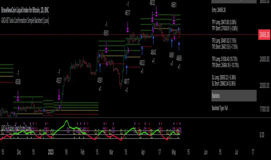
[Fedra Algotrading Strategy]English / Spanish
Algotrading strategy optimized for cryptocurrencies. Originally conceived to trade automatically through bots (that's how I use it), it also works to get signals and trade manually in any exchange.
It works in spot. It does not repaint. Works in 15M, 30M, 1H and 4H (I prefer short periods).
Features:
Buy the dip:
Attempts to buy on the dip, finding entries when the price makes abrupt dips that break the linear regression of the last periods (default 40).
Trailing Take Profit:
Once the percentage established for the take profit is reached, the strategy follows the price if it is rising until it stops rising and only then makes the sale.
Trend Detection:
Determines whether the market is in an uptrend or downtrend by crossing 2 SMAs. This affects the performance of the strategy. This works as a filter to avoid making entries in a downtrend.
Trailing Break Even:
If the market enters a downtrend with an open trade, a Trailing Break Even is triggered, (configurable, default 1.5%). The intention is to close the trade as soon as possible, but without losses. The value of 1.5% is intended to cover commission costs and a possible spread. Like the Take Profit, the Trailing Break Even follows the price as it rises until it stops doing so before closing the trade.
How to use this strategy?
In the properties of the strategy you assign the amount you will trade (default 100), the percentage of the total capital you will use in each trade (default 100%) and the value of the commissions (default 1%).
Select the pair to trade. The strategy is optimized for trading pairs with stable coins. The strategy benefits from volatility so choosing among currencies with a market cap between 50M and 10,000M gives better profits than with top 10 currencies.
In the strategy options, disable the stoploss by setting it to 100% to be able to concentrate on the Take Profit.
With an eye on the "Net Profit" of the strategy, start with the take profit at 3% (for lower percentages there is the Break Even) and increase it 1 by 1 until determining which is the best for our pair (the one that gives us a better net profit).
Once the Take Profit is established, enable the StopLoss starting from 1 and choosing the best parameter looking for the balance that makes us feel comfortable between the Net Profit and the total of closed operations.
Test this same with candles of different periods (I trade with 15M and 30M candles).
Tip:
To trade automatically using a bot, I recommend using pairs in which the strategy has a profitability higher than 80%.
To counteract possible overfitting, when the strategy has given me a 30% profit, I recalculate the optimal parameters.
If you are interested in auromatizing it to trade on Binance, Binance US, AAX, Kucoin, Liquid, Okex, Bitfinex, Bittrex, Coinbase Pro, Gemini, HitBTC, Kraken or Poloniex, I recommend using Quadency bots, they are free and the ones I use.
This will eventually be a paid script, but you can request free access for now.
I am still working on optimizations, improvements, and more features.
DCA version coming soon.
I leave some optimizations of the spares I am trading at the moment (On 15M candles):
PAIR SL TP Bars Profit Profit Rentability
OM 3 4 96 70 2703.41% 88.57%
NU 4 3 96 81 1170.38% 86.42%
ONE 4 4 192 83 756% 91.57%
FTM 8 4 192 80 900.00% 92.50%
LUNA 3 8 192 78 410.98% 83.33%
OMG 6 4 192 72 408.75% 88.89%
FRONT 2 5 96 61 406% 85.25%
SOL 5 10 96 84 381.78% 83.33%
UTK 2 4 192 59 520.00% 88.06%
NMR 2 3 96 76 279% 80.26%
STPT 1 4 96 84 272.34% 79.76%
ROSE 5 4 96 59 478.00% 88.00%
clv 4 5 192 46 216% 78.26%
XTZ 4 6 96 87 216.00% 82.76%
C98 1 6 96 36 184.46% 80.56%
ALGO 7 4 192 61 222.00% 88.52%
ATOM 6 4 96 73 160.40% 86.30%
DOT 3 6 96 75 156.54% 84%
REEF 4 4 96 67 154.90% 85.07%
AUDIO 10 5 192 62 128.48% 83.87%
DYDX 1 10 96 20 120.76% 90%
DOT 4 6 96 77 111.33% 83.12%
KEEP 7 5 96 69 110% 87%
MINA 7 6 96 23 100.29% 86.96%
OPUL 1 5 96 18 95.26% 100%
HBAR 1 3 192 76 91.82% 81.58%
VRA/USDT 7 4 96 81 89.35% 81.48%
XEC 3 14 96 27 89.24% 85.19%
*****************************************************SPANISH*****************************************
Estrategia de Algotrading optimizada para criptomonedas. Originalmente concebida para operar de manera automática mediante bots (así la utilizo yo), funciona también para obtener señales y operar manualmente en cualquier exchange.
Funciona en spot. No repinta. Funciona en 15M, 30M, 1H y 4H (Yo prefiero periodos cortos)
Características:
Buy the dip:
Intenta comprar en el dip, encontrando entradas cuando el precio hace bajadas abruptas que rompen la regresión lineal de los últimos periodos (por defecto 40)
Trailing Take Profit:
Una vez alcanzado el porcentaje establecido para el take profit, la estrategia acompaña al precio si está en ascenso hasta que deja de subir y recién ahí realiza la venta.
Detección de Trend:
Determina si el mercado tiene una tendencia alcista o bajista mediante el cruce de 2 SMAs. Esto afecta el funcionamiento de la estrategia. Esto funciona como filtro para evitar realizar entradas en una tendencia bajista.
Trailing Break Even:
Si el mercado entra en tendencia bajista con una operación abierta, se activa un Trailing Break Even, (configurable, por defecto 1.5%). La intención es cerrar la operación lo antes posible, pero sin pérdidas. El valor de 1.5% está pensado para cubrir los costos de comisiones y un posible spread. Al igual que el Take Profit, El Trailing Break Even acompaña al precio mientras sube hasta que deja de hacerlo antes de cerrar la operación.
Cómo utilizar esta estrategia?
En las propiedades de la estrategia se le asigna el monto con el que va a operar (por defecto 100), el porcentaje del total de capital que utilizará en cada operación (por defecto 100%) y el valor de las comisiones (por defecto 1%)
Seleccionar el par a operar. La estrategia está optimizada para operar en pares con stablecoins. La estrategia se beneficia con la volatilidad por lo que elegir entre las monedas con un market cap de entre 50M y 10.000M da mejores beneficios que con monedas del top 10
En las opciones de la estrategia, deshabilitar el stoploss configurándolo en 100% para poder concentrarnos en el Take Profit.
Con un ojo en el “Beneficio Neto” de la estrategia, comenzar con el take profit en 3% (para porcentajes menores está el Break Even) e ir aumentándolo de 1 en 1 hasta determinar cuál es el mejor para nuestro par (el que nos proporciona un major beneficio neto).
Establecido el Take Profit, habilitar el StopLoss partiendo de 1 y eligiendo el mejor parámetro buscando el equilibrio que nos haga sentir cómodos entre el Beneficio Neto y el total de operaciones cerradas.
Probar esto mismo con velas de diferentes periodos (Yo opero con velas de 15M y 30M)
Consejo:
Para operar de manera automática mediante un bot, recomiendo utilizar pares en los que la estrategia tenga una rentabilidad superior al 80%
Para contrarestar posible overfiting, cuando la estrategia me ha dado un 30% de profit, vuelvo a calcular los parámetros óptimos.
Si te interesa auromatizarla para operar en Binance, Binance US, AAX, Kucoin, Liquid, Okex, Bitfinex, Bittrex, Coinbase Pro, Gemini, HitBTC, Kraken o Poloniex, recomiendo usar los bots de Quadency, son gratiutos y los que yo utilizo.
Este será eventualmente un script pago, pero puedes solicitar acceso gratuito por ahora.
Sigo trabajando en optimizaciones, mejoras, y más funciones.
Próximamente versión DCA.
Dejo algunas optimizaciones de lo spares que yo estoy operando en este momento (En velas de 15M contra BUSD):
PAR SL TP Bars Operaciones Profit Rentabilidad
OM 3 4 96 70 2703.41% 88.57%
NU 4 3 96 81 1170.38% 86.42%
ONE 4 4 192 83 756% 91.57%
FTM 8 4 192 80 900.00% 92.50%
LUNA 3 8 192 78 410.98% 83.33%
OMG 6 4 192 72 408.75% 88.89%
FRONT 2 5 96 61 406% 85.25%
SOL 5 10 96 84 381.78% 83.33%
UTK 2 4 192 59 520.00% 88.06%
NMR 2 3 96 76 279% 80.26%
STPT 1 4 96 84 272.34% 79.76%
ROSE 5 4 96 59 478.00% 88.00%
clv 4 5 192 46 216% 78.26%
XTZ 4 6 96 87 216.00% 82.76%
C98 1 6 96 36 184.46% 80.56%
ALGO 7 4 192 61 222.00% 88.52%
ATOM 6 4 96 73 160.40% 86.30%
DOT 3 6 96 75 156.54% 84%
REEF 4 4 96 67 154.90% 85.07%
AUDIO 10 5 192 62 128.48% 83.87%
DYDX 1 10 96 20 120.76% 90%
DOT 4 6 96 77 111.33% 83.12%
KEEP 7 5 96 69 110% 87%
MINA 7 6 96 23 100.29% 86.96%
OPUL 1 5 96 18 95.26% 100%
HBAR 1 3 192 76 91.82% 81.58%
VRA/USDT 7 4 96 81 89.35% 81.48%
XEC 3 14 96 27 89.24% 85.19%

Multi-Market Swing Trader Webhook Ready [HullBuster]
Introduction
This is an all symbol swing trading strategy intended for webhook integration to live accounts. This script employs an adjustable bandwidth ping pong algorithm which can be run in long only, short only or bidirectional modes. Additionally, this script provides advanced features such as pyramiding and DCA. It has been in development for nearly three years and exposes over 90 inputs to accommodate varying risk reward ratios. Equipped with a proper configuration it is suitable for professional traders seeking quality trades from a cloud based platform. This is my most advanced Pine Script to date which combines my RangeV3 and TrendV2 scripts. Using this combination it tries to bridge the gap between range bound and trending markets. I have put a lot of time into creating a system that could transition by itself so as to require less human intervention and thus be able to withstand long periods in full automation mode.
As a Pine strategy, hypothetical performance can be easily back-tested. Allowing you to Iron out the configuration of your target instrument. Now with recent advancements from the Pine development team this same script can be connected to a webhook through the alert mechanism. The requirement of a separate study script has been completely removed. This really makes things a lot easier to get your trading system up and running. I would like to also mention that TradingView has made significant advancements to the back-end over the last year. Notably, compile times are much faster now permitting more complex algorithms to be implemented. Thank you TradingView!
I used QuantConnect as my role model and strived to produce a base script which could compete with higher end cloud based platforms while being attractive to similarly experienced traders. The versatility of the Pine Language combined with the greater selection of end point execution systems provides a powerful alternative to other cloud based platforms. At the very least, with the features available today, a modular trading system for everyday use is a reality. I hope you'll agree.
This is a swing trading strategy so the behavior of this script is to buy on weakness and sell on strength. In trading parlance this is referred to as Support and Resistance Trading. Support being the point at which prices stop falling and start rising. Resistance being the point at which prices stop rising and fall. The chart real estate between these two points being defined as the range. This script seeks to implement strategies to profit from placing trades within this region. Short positions at resistance and long positions at support. Just to be clear, the range as well as trends are merely illusions as the chart only receives prices. However, this script attempts to calculate pivot points from the price stream. Rising pivots are shorts and falling pivots are longs. I refer to pivots as a vertex in this script which adds structural components to the chart formation (point, sides and a base). When trading in “Ping Pong” mode long and short positions are interleaved continuously as long as there exists a detectable vertex.
This is a non-hedging script so those of us subject to NFA FIFO Rule 2-43(b) should be generally safe to webhook into signals emitted from this script. However, as covered later in this document, there are some technical limitations to this statement. I have tested this script on various instruments for over two years and have configurations for forex, crypto and stocks. This script along with my TrendV2 script are my daily trading vehicles as a webhook into my forex and crypto accounts. This script employs various high risk features that could wipe out your account if not used judiciously. You should absolutely not use this script if you are a beginner or looking for a get-rich-quick strategy. Also please see my CFTC RULE 4.41 disclosure statement at the end of the document. Really!
Does this script repaint? The short answer is yes, it does, despite my best efforts to the contrary. EMAs are central to my strategy and TradingView calculates from the beginning of the series so there is just no getting around this. However, Pine is improving everyday and I am hopeful that this issue will be address from an architectural level at some point in the future. I have programmed my webhook to compensate for this occurrence so, in the mean time, this my recommended way to handle it (at the endpoint and before the broker).
Design
This strategy uses a ping pong algorithm of my own design. Basically, trades bounce off each other along the price stream. Trades are produced as a series of reversals. The point at which a trade reverses is a pivot calculation. A measurement is made between the recent valley to peak which results in a standard deviation value. This value is an input to implied probability calculation.Yes, the same implied probability used in sports betting. Odds are then calculated to determine the likelihood of price action continuing or retracing to the pivot. Based on where the account is at alert time, the action could be an entry, take profit or pyramid signal. In this design, trades must occur in alternating sequence. A long followed by a short then another long followed by a short and so on. In range bound price action trades appear along the outer bands of the channel in the aforementioned sequence. Shorts on the top and longs at the bottom. Generally speaking, the widths of the trading bands can be adjusted using the vertex dynamics in Section 2. There are a dozen inputs in this section used to describe the trading range. It is not a simple adjustment. If pyramids are enabled the strategy overrides the ping pong reversal pattern and begins an accumulation sequence. In this case you will see a series of same direction trades.
This script uses twelve indicators on a single time frame. The original trading algorithms are a port from a C++ program on proprietary trading platform. I’ve converted some of the statistical functions to use standard indicators available on TradingView. The setups make heavy use of the Hull Moving Average in conjunction with EMAs that form the Bill Williams Alligator as described in his book “New Trading Dimensions” Chapter 3. Lag between the Hull and the EMAs play a key role in identifying the pivot points. I really like the Hull Moving Average. I use it in all my systems, including 3 other platforms. It’s is an excellent leading indicator and a relatively light calculation.
The trend detection algorithms rely on several factors:
1. Smoothed EMAs in a Willams Alligator pattern.
2. Number of pivots encountered in a particular direction.
3. Which side debt is being incurred.
4. Settings in Section 4 and 5 (long and short)
The strategy uses these factors to determine the probability of prices continuing in the most recent direction. My TrendV2 script uses a higher time frame to determine trend direction. I can’t use that method in this script without exceeding various TradingView limitations on code size. However, the higher time frame is the best way to know which trend is worth pursuing or better to bet against.
The entire script is around 2400 lines of Pine code which pushes the limits of what can be created on this platform given the TradingView maximums for: local scopes, run-time duration and compile time. The module has been through numerous refactoring passes and makes extensive use of ternary statements. As such, It takes a full minute to compile after adding it to a chart. Please wait for the hovering dots to disappear before attempting to bring up the input dialog box. Scrolling the chart quickly may bring up an hour glass.
Regardless of the market conditions: range or trend. The behavior of the script is governed entirely by the 91 inputs. Depending on the settings, bar interval and symbol, you can configure a system to trade in small ranges producing a thousand or more trades. If you prefer wider ranges with fewer trades then the vertex detection settings in Section 2 should employ stiffer values. To make the script more of a trend follower, adjustments are available in Section 4 and 5 (long and short respectively). Overall this script is a range trader and the setups want to get in that way. It cannot be made into a full blown trend trading system. My TrendV2 is equipped for that purpose. Conversely, this script cannot be effectively deployed as a scalper either. The vertex calculation require too much data for high frequency trading. That doesn’t work well for retail customers anyway. The script is designed to function in bar intervals between 5 minutes and 4 hours. However, larger intervals require more backtest data in order to create reliable configurations. TradingView paid plans (Pro) only provide 10K bars which may not be sufficient. Please keep that in mind.
The transition from swing trader to trend follower typically happens after a stop is hit. That means that your account experiences a loss first and usually with a pyramid stack so the loss could be significant. Even then the script continues to alternate trades long and short. The difference is that the strategy tries to be more long on rising prices and more short on falling prices as opposed to simply counter trend trading. Otherwise, a continuous period of rising prices results in a distinctly short pyramid stack. This is much different than my TrendV2 script which stays long on peaks and short on valleys. Basically, the plan is to be profitable in range bound markets and just lose less when a trend comes along. How well this actually plays out will depend largely on the choices made in the sectioned input parameters.
Sections
The input dialog for this script contains 91 inputs separated into six sections.
Section 1: Global settings for the strategy including calculation model, trading direction, exit levels, pyramid and DCA settings. This is where you specify your minimum profit and stop levels. You should setup your Properties tab inputs before working on any of the sections. It’s really important to get the Base Currency right before doing any work on the strategy inputs. It is important to understand that the “Minimum Profit” and “Limit Offset” are conditional exits. To exit at a profit, the specified value must be exceeded during positive price pressure. On the other hand, the “Stop Offset” is a hard limit.
Section 2: Vertex dynamics. The script is equipped with four types of pivot point indicators. Histogram, candle, fractal and transform. Despite how the chart visuals may seem. The chart only receives prices. It’s up to the strategy to interpret patterns from the number stream. The quality of the feed and the symbol’s bar characteristics vary greatly from instrument to instrument. Each indicator uses a fundamentally different pattern recognition algorithm. Use trial and error to determine the best fit for your configuration. After selecting an indicator type, there are eight analog fields that must be configured for that particular indicator. This is the hardest part of the configuration process. The values applied to these fields determine how the range will be measured. They have a big effect on the number of trades your system will generate. To see the vertices click on the “Show Markers” check box in this section. Red markers are long positions and blue markers are short. This will give you an idea of where trades will be placed in natural order.
Section 3: Event thresholds. Price spikes are used to enter and exit trades. The magnitude which define these spikes are configured here. The rise and fall events are primarily for pyramid placement. The rise and fall limits determine the exit threshold for the conditional “Limit Offset” field found in Section 1. These fields should be adjusted one at a time. Use a zero value to disengage every one but the one you are working on. Use the fill colors found in Section 6 to get a visual on the values applied to these fields. To make it harder for pyramids to enter stiffen the Event values. This is more of a hack as the formal pyramid parameters are in Section 1.
Section 4 and 5: Long and short settings. These are mirror opposite settings with all opposing fields having the same meaning. Its really easy to introduce data mining bias into your configuration through these fields. You must combat against this tendency by trying to keep your settings as uniform as possible. Wildly different parameters for long and short means you have probably fitted the chart. There are nine analog and thirteen Boolean fields per trade direction. This section is all about how the trades themselves will be placed along the range defined in Section 2. Generally speaking, more restrictive settings will result in less trades but higher quality. Remember that this strategy will enter long on falling prices and short on rising prices. So getting in the trade too early leads to a draw-down. However, this could be what you want if pyramiding is enabled. I, personally, have found that the best configurations come from slightly skewing one side. I just accept that the other side will be sub-par.
Section 6: Chart rendering. This section contains one analog and four Boolean fields. More or less a diagnostic tool. Of particular interest is the “Symbol Debt Sequence” field. This field contains a whole number which paints regions that have sustained a run of bad trades equal or greater than specified value. It is useful when DCA is enabled. In this script Dollar Cost Averaging on new positions continues only until the symbol debt is recouped. To get a better understanding on how this works put a number in this field and activate DCA. You should notice how the trade size increases in the colored regions. The “Summary Report” checkbox displays a blue information box at the live end of the chart. It exposes several metrics which you may find useful if manually trading this strategy from audible alerts or text messages.
Pyramids
This script features a downward pyramiding strategy which increases your position size on losing trades. On purely margin trades, this feature can be used to, hypothetically, increase the profit factor of positions (not individual trades). On long only markets, such as crypto, you can use this feature to accumulate coins at depressed prices. The way it works is the stop offset, applied in the Section 1 inputs, determines the maximum risk you intend to bear. Additional trades will be placed at pivot points calculated all the way down to the stop price. The size of each add on trade is increased by a multiple of its interval. The maximum number of intervals is limited by the “Pyramiding” field in the properties tab. The rate at which pyramid positions are created can be adjusted in Section 1. To see the pyramids click on the “Mark Pyramid Levels” check box in the same section. Blue triangles are painted below trades other than the primary.
Unlike traditional Martingale strategies, the result of your trade is not dependent on the profit or loss from the last trade. The position must recover the R1 point in order to close. Alternatively, you can set a “Pyramid Bale Out Offset” in Section 1 which will terminate the trade early. However, the bale out must coincide with a pivot point and result in a profitable exit in order to actually close the trade. Should the market price exceed the stop offset set in Section 1, the full value of the position, multiplied by the accepted leverage, will be realized as a loss to the trading account. A series of such losses will certainly wipe out your account.
Pyramiding is an advanced feature intended for professional traders with well funded accounts and an appropriate mindset. The availability of this feature is not intended to endorse or promote my use of it. Use at your own risk (peril).
DCA
In addition to pyramiding this script employs DCA which enables users to experiment with loss recovery techniques. This is another advanced feature which can increase the order size on new trades in response to stopped out or winning streak trades. The script keeps track of debt incurred from losing trades. When the debt is recovered the order size returns to the base amount specified in the properties tab. The inputs for this feature are found in section 3 and include a limiter to prevent your account from depleting capital during runaway markets. The main difference between DCA and pyramids is that this implementation of DCA applies to new trades while pyramids affect open positions. DCA is a popular feature in crypto trading but can leave you with large “bags” if your not careful. In other markets, especially margin trading, you’ll need a well funded account and much experience.
To be sure pyramiding and dollar cost averaging is as close to gambling as you can get in respectable trading exchanges. However, if you are looking to compete in a spot trading contest or just want to add excitement to your trading life style those features could find a place in your strategies. Although your backtest may show spectacular gains don’t expect your live trading account to do the same. Every backtest has some measure of data mining bias. Please remember that.
Webhook Integration
The TradingView alerts dialog provides a way to connect your script to an external system which could actually execute your trade. This is a fantastic feature that enables you to separate the data feed and technical analysis from the execution and reporting systems. Using this feature it is possible to create a fully automated trading system entirely on the cloud. Of course, there is some work to get it all going in a reliable fashion. To that end this script has several things going for it. First off, it is a strategy type script. That means that the strategy place holders such as {{strategy.position_size}} can be embedded in the alert message text. There are more than 10 variables which can write internal script values into the message for delivery to the specified endpoint. Additionally, my scripts output the current win streak and debt loss counts in the {{strategy.order.alert_message}} field. Depending on the condition, this script will output other useful values in the JSON “comment” field of the alert message. Here is an excerpt of the fields I use in my webhook signal:
"broker_id": "kraken",
"account_id": "XXX XXXX XXXX XXXX",
"symbol_id": "XMRUSD",
"action": "{{strategy.order.action}}",
"strategy": "{{strategy.order.id}}",
"lots": "{{strategy.order.contracts}}",
"price": "{{strategy.order.price}}",
"comment": "{{strategy.order.alert_message}}",
"timestamp": "{{time}}"
Though TradingView does a great job in dispatching your alert this feature does come with a few idiosyncrasies. Namely, a single transaction call in your script may cause multiple transmissions to the endpoint. If you are using placeholders each message describes part of the transaction sequence. A good example is closing a pyramid stack. Although the script makes a single strategy.close() call, the endpoint actually receives a close message for each pyramid trade. The broker, on the other hand, only requires a single close. The incongruity of this situation is exacerbated by the possibility of messages being received out of sequence. Depending on the type of order designated in the message, a close or a reversal. This could have a disastrous effect on your live account. This broker simulator has no idea what is actually going on at your real account. Its just doing the job of running the simulation and sending out the computed results. If your TradingView simulation falls out of alignment with the actual trading account lots of really bad things could happen. Like your script thinks your are currently long but the account is actually short. Reversals from this point forward will always be wrong with no one the wiser. Human intervention will be required to restore congruence. But how does anyone find out this is occurring? In closed systems engineering this is known as entropy. In practice your webhook logic should be robust enough to detect these conditions. Be generous with the placeholder usage and give the webhook code plenty of information to compare states. Both issuer and receiver. Don’t blindly commit incoming signals without verifying system integrity.
Operation
This is a swing trading strategy so the fundamental behavior of this script is to buy on weakness and sell on strength. As such trade orders are placed in a counter direction to price pressure. What you will see on the chart is a short position on peaks and a long position on valleys. This is slightly misleading since a range as well as a trend are best recognized, in hindsight, after the patterns occur on the chart. In the middle of a trade, one never knows how deep valleys will drop or how high peaks will rise. For certain, long trades will continue to trigger as the market prices fall and short trades on rising prices. This means that the maximum efficiency of this strategy is achieved in choppy markets where the price doesn’t extend very far from its adjacent pivot point. Conversely, this strategy will be the least efficient when market conditions exhibit long continuous single direction price pressure. Especially, when measured in weeks. Translation, the trend is not your friend with this strategy. Internally, the script attempts to recognize prolonged price pressure and changes tactics accordingly. However, at best, the goal is to weather the trend until the range bound market returns. At worst, trend detection fails and pyramid trades continue to be placed until the limit specified in the Properties tab is reached. In all likelihood this could trigger a margin call and if it hits the stop it could wipe out your account.
This script has been in beta test four times since inception. During all that time no one has been successful in creating a configuration from scratch. Most people give up after an hour or so. To be perfectly honest, the configuration process is a bear. I know that but there is no way, currently, to create libraries in Pine. There is also no way specify input parameters other than the flattened out 2-D inputs dialog. And the publish rules clearly state that script variations addressing markets or symbols (suites) are not permitted. I suppose the problem is systemic to be-all-end-all solutions like my script is trying to be. I needed a cloud strategy for all the symbols that I trade and since Pine does not support library modules, include files or inter process communication this script and its unruly inputs are my weapon of choice in the war against the market forces. It takes me about six hours to configure a new symbol. Also not all the symbols I configure are equally successful. I should mention that I have a facsimile of this strategy written in another platform which allows me to run a backtest on 10 years of historical data. The results provide me a sanity check on the inputs I select on this platform.
My personal configurations use a 10 minute bar interval on forex instruments and 15 minutes on crypto. I try to align my TradingView scripts to employ standard intervals available from the broker so that I can backtest longer durations than those available on TradingView. For example, Bitcoin at 15 minute bars is downloadable from several sources. I really like the 10 minute bar. It provides lots of detectable patterns and is easy to store many years in an SQL database.
The following steps provide a very brief set of instructions that will get you started but will most certainly not produce the best backtest. A trading system that you are willing to risk your hard earned capital will require a well crafted configuration that involves time, expertise and clearly defined goals. As previously mentioned, I have several example configurations that I use for my own trading that I can share with you if you like. To get hands on experience in setting up your own symbol from scratch please follow the steps below.
Step 1. Setup the Base currency and order size in the properties tab.
Step 2. Select the calculation presets in the Instrument Type field.
Step 3. Select “No Trade” in the Trading Mode field
Step 4. Select the Histogram indicator from Section 2. You will be experimenting with different ones so it doesn’t matter which one you try first.
Step 5. Turn on Show Markers in Section 2.
Step 6. Go to the chart and checkout where the markers show up. Blue is up and red is down. Long trades show up along the red markers and short trades on the blue.
Step 7. Make adjustments to “Base To Vertex” and “Vertex To Base” net change and ROC in Section 2. Use these fields to move the markers to where you want trades to be.
Step 8. Try a different indicator from Section 2 and repeat Step 7 until you find the best match for this instrument on this interval. This step is complete when the Vertex settings and indicator combination produce the most favorable results.
Step 9. Go to Section 4 and enable “Apply Red Base To Base Margin”.
Step 10. Go to Section 5 and enable “Apply Blue Base To Base Margin”.
Step 11. Go to Section 2 and adjust “Minimum Base To Base Blue” and “Minimum Base To Base Red”. Observe the chart and note where the markers move relative to each other. Markers further apart will produce less trades but will reduce cutoffs in “Ping Pong” mode.
Step 12. Turn off Show Markers in Section 2.
Step 13. Put in your Minimum Profit and Stop Loss in the first section. This is in pips or currency basis points (chart right side scale). Percentage is not currently supported. Note that the profit is taken as a conditional exit on a market order not a fixed limit. The actual profit taken will almost always be greater than the amount specified. The stop loss, on the other hand, is indeed a hard number which is executed by the TradingView broker simulator when the threshold is breached.
Step 14. Return to step 3 and select a Trading Mode (Long, Short, BiDir, Ping Pong). If you are planning to trade bidirectionally its best to configure long first then short. Combine them with “BiDir” or “Ping Pong” after setting up both sides of the trade individually. The difference between “BiDir” and “Ping Pong” is that “Ping Pong” uses position reversal and can cut off opposing trades less than the specified minimum profit. As a result “Ping Pong” mode produces the greatest number of trades.
Step 15. Take a look at the chart. Trades should be showing along the markers plotted earlier.
Step 16. Make adjustments to the Vertex fields in Section 2 until the TradingView performance report is showing a profit. This includes the “Minimum Base To Base” fields. If a profit cannot be achieved move on to Step 17.
Step 17. Improve the backtest profitability by adjusting the “Entry Net Change” and “Entry ROC” in Section 4 and 5.
Step 18. Enable the “Mandatory Snap” checkbox in Section 4 and 5 and adjust the “Snap Candle Delta” and “Snap Fractal Delta” in Section 2. This should reduce some chop producing unprofitable reversals.
Step 19. Increase the distance between opposing trades by adding an “Interleave Delta” in Sections 4 and 5. This is a floating point value which starts at 0.01 and typically does not exceed 2.0.
Step 20. Increase the distance between opposing trades even further by adding a “Decay Minimum Span” in Sections 4 and 5. This is an absolute value specified in the symbol’s quote currency (right side scale of the chart). This value is similar to the minimum profit and stop loss fields in Section 1.
Step 21. The “Buy Composite Strength” input works in tandem with “Long Decay Minimum Span” in Section 4. Try enabling and see if it improves the performance. This field is only relevant when there is a value in “Long Decay Minimum Span”.
Step 22. The “Sell Composite Weakness” input works in tandem with “Short Decay Minimum Span” in Section 5. Try enabling and see if it improves the performance. This field is only relevant when there is a value in “Short Decay Minimum Span”.
Step 23. Improve the backtest profitability by adjusting the “Adherence Delta” in Section 4 and 5. This field requires the “Adhere to Rising Trend” checkbox to be enabled.
Step 24. At this point your strategy should be more or less working. Experiment with the remaining check boxes in Section 4 and 5. Keep the ones which seem to improve the performance.
Step 25. Examine the chart and see that trades are being placed in accordance with your desired trading goals. This is an important step. If your desired model requires multiple trades per day then you should be seeing hundreds of trades on the chart. Alternatively, you may be looking to trade fewer steep peaks and deep valleys in which case you should see trades at major turning points. Don’t simply settle for what the backtest serves you. Work your configuration until the system aligns with your desired model. Try changing indicators and even intervals if you cannot reach your simulation goals. Generally speaking, the histogram and Candle indicators produce the most trades. The Fractal indicator captures the tallest peaks and valleys. The Transform indicator is the most reliable but doesn’t well work on all instruments.
Example Settings
To reproduce the performance shown on the chart please use the following configuration:
1. Select XBTUSD Kraken as the chart symbol.
2. On the properties tab set the Order Size to: 0.01 Bitcoin
3. On the properties tab set the Pyramiding to: 10
4. In Section 1: Select “Forex” for the Instrument Type
5. In Section 1: Select “Ping Pong” for the Trading Mode
6. In Section 1: Input 1200 for the Minimum Profit
7. In Section 1: Input 15000 for the Stop Offset
8. In Section 1: Input 1200 for the Pyramid Minimum Span
9. In Section 1: Check mark the Ultra Wide Pyramids
10. In Section 2: Check mark the Use Transform Indicator
So to be clear, I used a base position size of one - one hundredth of a Bitcoin and allow the script to add up to 10 downward pyramids. The example back-test did hit eight downward pyramids. That means the account would have to be able to withstand a base position size (0.01) times 28. The resulting position size is 0.28 of a Bitcoin. If the price of Bitcoin is 35K then the draw down amount (not including broker fees) would be $9800 dollars. Since I have a premium subscription my backtest chart includes 20K historical bars. That's roughly six months of data. As of today, pro accounts only get 10K bars so the performance cannot be exactly matched with such a difference in historical data. Please keep that in mind.
There are, of course, various ways to reduce the risk incurred from accumulating pyramids. You can increase the “Pyramid Minimum Span” input found in Section 2 which increases the space between each pyramid trade. Also you can set a “Pyramid Bale Out Offset” in the same input section. This lets you out of the trade faster on position recovery. For example: Set a value of 8000 into this input and the number of trades increase to 178 from 157. Since the positions didn’t go full term, more trades were created at less profit each. The total brute force approach would be to simply limit the number of pyramids in the Properties tab.
It should be noted that since this is crypto, accumulating on the long side may be what you want. If you are not trading on margin and thus outright buying coins on the Kraken exchange you likely are interested in increasing your Bitcoin position at depressed prices. This is a popular feature on some of the other crypto trading packages like CryptoHopper and Profit Trailer. Click on Enable TV Long Only Rule in Section 1. This switches the signal emitter to long only. However, you may still see short trades on the chart. They are treated as a close instead of a reversal.
Feel free to PM me with any questions related to this script. Thank you and happy trading!
CFTC RULE 4.41
These results are based on simulated or hypothetical performance results that have certain inherent limitations. Unlike the results shown in an actual performance record, these results do not represent actual trading. Also, because these trades have not actually been executed, these results may have under-or over-compensated for the impact, if any, of certain market factors, such as lack of liquidity. Simulated or hypothetical trading programs in general are also subject to the fact that they are designed with the benefit of hindsight. No representation is being made that any account will or is likely to achieve profits or losses similar to these being shown.
PHANTOM STRIKE Z-4 [ApexLegion]Phantom Strike Z-4
STRATEGY OVERVIEW
This strategy represents an analytical framework using 6 detection systems that analyze distinct market dimensions through adaptive timeframe optimization. Each system targets specific market inefficiencies - automated parameter adjustment, market condition filtering, phantom strike pattern detection, SR exit management, order block identification, and volatility-aware risk management - with results processed through a multi-component scoring calculation that determines signal generation and position management decisions.
SYSTEM ARCHITECTURE PHILOSOPHY
Phantom Strike Z-4 operates through 12 distinct parameter groups encompassing individual settings that allow detailed customization for different trading environments. The strategy employs modular design principles where each analytical component functions independently while contributing to unified decision-making protocols. This architecture enables traders to engage with structured market analysis through intuitive configuration options while the underlying algorithms handle complex computational processes.
The framework approaches certain aspects differently from static trading approaches by implementing real-time parameter adjustment based on timeframe characteristics, market volatility conditions, news event detection, and weekend gap analysis. During low-volatility periods where traditional strategies struggle to generate meaningful returns, Z-4's adaptive systems identify micro-opportunities through formation analysis and systematic patience protocols.
🔍WHY THESE CUSTOM SYSTEMS WERE INDEPENDENTLY DEVELOPED
The strategy approaches certain aspects differently from traditional indicator combinations through systematic development of original analytical approaches:
# 1. Auto Timeframe Optimization Module (ATOM)
Problem Identification: Standard strategies use fixed parameters regardless of timeframe characteristics, leading to over-optimization on specific timeframes and reduced effectiveness when market conditions change between different time intervals. Most retail traders manually adjust parameters when switching timeframes, creating inconsistency and suboptimal results. Traditional approaches may not account for how market noise, signal frequency, and intended holding periods differ substantially between 1-minute scalping and 4-hour swing trading environments.
Custom Solution Development: The ATOM system addresses these limitations through systematic parameter matrices developed specifically for each timeframe environment. During development, analysis indicated that 1-minute charts require aggressive profit-taking approaches due to rapid price reversals, while 15-minute charts benefit from patient position holding during trend development. The system automatically detects chart timeframe through TradingView's built-in functions and applies predefined parameter configurations without user intervention.
Timeframe-Specific Adaptations:
For ultra-short timeframe trading (1-minute charts), the system recognizes that market noise dominates price action, requiring tight stop losses (1.0%) and rapid profit realization (25% at TP1, 35% at TP2, 40% at TP3). Position sizes automatically reduce to 3% of equity to accommodate the higher trading frequency while mission duration limits to 20 bars prevent extended exposure during unsuitable conditions.
Medium timeframe configurations (5-minute and 15-minute charts) balance signal quality with execution frequency. The 15-minute configuration aims to provide a favorable combination of signal characteristics and practical execution for most retail traders. Formation thresholds increase to 2.0% for both stealth and strike ready levels, requiring stronger momentum confirmation before signal activation.
Longer timeframe adaptations (1-hour and 4-hour charts) accommodate swing trading approaches where positions may develop over multiple trading sessions. Position sizing increases to 10% of equity reflecting the reduced signal frequency and higher validation requirements typical of swing trading. Take profit targets extend considerably (TP1: 2.0%, TP2: 4.0%, TP3: 8.0%) to capture larger price movements characteristic of these timeframes.
# 2. Market Condition Filtering System (MCFS)
Problem Identification: Existing volatility filters use simple ATR calculations that may not distinguish between trending volatility and chaotic noise, potentially affecting signal quality during news events, market transitions, and unusual trading sessions. Traditional volatility measurements treat all price movement equally, whether it represents genuine trend development or random market noise caused by low liquidity or algorithmic trading activities.
Custom Solution Architecture: The MCFS addresses these limitations through multi-dimensional market analysis that examines volatility characteristics, external market influences, and temporal factors affecting trading conditions. Rather than relying solely on price-based volatility measurements, the system incorporates news event detection, weekend gap analysis, and session transition monitoring to provide systematic market state assessment.
Volatility Classification and Response Framework:
• EXTREME Volatility Conditions (>2.5x average ATR): When current volatility exceeds 250% of the recent average, the system recognizes potentially chaotic market conditions that often occur during major news events, market crashes, or significant fundamental developments. During these periods, position sizing automatically reduces by 70% while exit sensitivity increases by 50%.
• HIGH Volatility Conditions (1.8-2.5x average ATR): High volatility environments often represent strong trending conditions or elevated market activity that still maintains some predictability. Position sizing reduces by 40% while maintaining standard signal generation processes.
• NORMAL Volatility Conditions (1.2-1.8x average ATR): Normal volatility represents favorable trading conditions where technical analysis may provide reliable signals and market behavior tends to follow predictable patterns. All strategy parameters operate at standard settings.
• LOW Volatility Conditions (0.8-1.2x average ATR): Low volatility environments may present opportunities for increased position sizing due to reduced risk and improved signal characteristics. Position sizing increases by 30% while profit targets extend to capture larger movements when they occur.
• DEAD Volatility Conditions (<0.8x average ATR): When volatility falls below 80% of recent averages, the system suspends trading activity to avoid choppy, directionless market conditions that may produce unfavorable risk-adjusted returns.
# 3. Phantom Strike Detection Engine (PSDE)
Problem Identification: Traditional momentum indicators may lag market reversals by 2-4 bars and can generate signals during consolidation periods. Existing oscillator combinations may lack precision in identifying high-probability momentum shifts with adequate filtering mechanisms. Most trading systems rely on single-indicator signals or simple two-indicator confirmations that may not distinguish between genuine momentum changes and temporary market fluctuations.
Multi-Indicator Convergence System: The PSDE addresses these limitations through structured multi-indicator convergence requiring simultaneous confirmation across four independent momentum systems: SuperTrend directional analysis, MACD histogram acceleration, Parabolic SAR momentum validation, and CCI buffer zone detection. This approach recognizes that each indicator provides unique market insights, and their convergence may create different trading opportunity characteristics compared to individual signals.
Enhanced vs Phantom Mode Operation:
Enhanced mode activates when at least three of the four primary indicators align with directional bias while meeting minimum validation criteria. Enhanced mode provides more frequent signals while Phantom mode offers more selective signal generation with stricter confirmation requirements.
Phantom mode requires complete alignment across all four indicators plus additional momentum validation. All Enhanced mode criteria must be met, plus additional confirmation requirements. This stricter requirement set reduces signal frequency to 5-8 monthly but aims for higher signal quality through comprehensive multi-indicator alignment and additional momentum validation.
# 4. Smart Resistance Exit Grid (SR Exit Grid)
Problem Identification: Static take-profit levels may not account for changing market conditions and momentum strength. Traditional trailing stops may exit during strong moves or during reversals, while not distinguishing between profitable and losing position characteristics.
Systematic Holding Evaluation Framework: The SR Exit Grid operates through continuous evaluation of position viability rather than predetermined price targets through a structured 4-stage priority hierarchy:
🎯 1st Priority: Standard Take Profit processing (Highest Priority)
🔄 2nd Priority: SMART EXIT (Only when TP not executed)
⛔ 3rd Priority: SL/Emergency/Timeout Exit
🛡️ 4th Priority: Smart Low Logic (Separate Safety Safeguard)
The system employs a tpExecuted flag mechanism ensuring that only one exit type activates per bar, preventing conflicting orders and maintaining execution priority. Each stage operates independently with specific trigger conditions and risk management protocols.
Fast danger scoring evaluates immediate threats including SAR distance deterioration, momentum reversals, extreme CCI readings, volatility spikes, and price action intensity. When combined scores exceed specified thresholds (8.0+ danger with <2.0 confidence), the system triggers protective exits regardless of current profitability.
# 5. Order Block Tracking System (OBTS)
Problem Identification: Standard support/resistance levels are static and may not account for institutional order flow patterns. Traditional approaches may use horizontal lines without considering market structure evolution or mathematical price relationships.
Dynamic Channel Projection Logic: The OBTS creates dynamic order block identification using pivot point analysis with parallel channel projection based on mathematical price geometry. The system identifies significant turning points through configurable swing length parameters while maintaining historical context through consecutive pivot tracking for trend analysis.
Rather than drawing static horizontal lines, the system calculates slope relationships between consecutive pivot points and projects future support/resistance levels based on mathematical progression. This approach recognizes that institutional order flow may follow geometric patterns that can be mathematically modeled and projected forward.
# 6. Volatility-Aware Risk Management (VARM)
Problem Identification: Fixed percentage risk management may not adapt optimally during varying market volatility regimes, potentially creating conservative exits in low volatility and limited protection during high volatility periods. Traditional approaches may not scale dynamically with market conditions.
Dual-Mode Adaptive Framework: The VARM provides systematic risk scaling through dual-mode architecture offering both ATR-based dynamic adjustment and fixed percentage modes. Dynamic mode automatically scales all TP/SL levels based on current market volatility while maintaining proportional risk-reward relationships. Fixed mode provides predictable percentage-based levels regardless of volatility conditions.
Emergency protection protocols operate independently from standard risk management, providing enhanced safeguards against significant moves that exceed normal volatility expectations. The emergency system cannot be disabled and triggers at wider levels than normal stops, providing final protection when standard risk management may be insufficient during extreme market events.
## Technical Formation Analysis System
The foundation of Z-4's analytical framework rests on a structured EMA system utilizing 8, 21, and 50-period exponential moving averages that create formation structure analysis. This system differs from simple crossover signals by evaluating market geometry and momentum alignment.
Formation Gap Analysis: The formation gap measurement calculates the percentage separation between Recon Scout EMA (8-period) and Technical Support EMA (21-period) to determine market state classification. When gap percentage falls below the Stealth Mode Threshold (default 1.5%), the market enters consolidation phase requiring enhanced patience. When gap exceeds Strike Ready Threshold (1.5%), conditions become favorable for momentum-based entries.
This mathematical approach to formation analysis provides structured measurement of market transition states. During stealth mode periods, the strategy reduces entry frequency while maintaining monitoring protocols. Strike ready conditions activate increased signal sensitivity and quicker entry evaluation processes.
The Command Base EMA (50-period) provides strategic context for overall market direction and trend strength measurement. Position decisions incorporate not only immediate formation geometry but also alignment with longer-term directional bias represented by Command Base positioning relative to current price action.
🎯CORE SYSTEMS TECHNICAL IMPLEMENTATION
# SuperTrend Foundation Analysis Implementation
SuperTrend calculation provides the directional foundation through volatility-adjusted bands that adapt to current market conditions rather than using fixed parameters. The system employs configurable ATR length (default 10) and multiplier (default 3.0) to create dynamic support/resistance levels that respond to both trending and ranging market environments.
Volatility-Adjusted Band Calculation:
st_atr = ta.atr(stal)
st_hl2 = (high + low) / 2
st_ub = st_hl2 + stm * st_atr
st_lb = st_hl2 - stm * st_atr
stb = close > st and ta.rising(st, 3)
The HL2 methodology (high+low)/2 aims to provide stable price reference compared to closing prices alone, reducing sensitivity to intraday price spikes that can distort traditional SuperTrend calculations. ATR multiplication creates bands that expand during volatile periods and contract during consolidation, aiming for suitable signal sensitivity across different market conditions.
Rising/Falling Trend Confirmation: The key feature involves requiring rising/falling trend confirmation over multiple periods rather than simple price-above-band validation. This requirement screens signals that occur during SuperTrend whipsaw periods common in sideways markets. SuperTrend signals with 3-period rising confirmation help reduce false signals that occur during sideways market conditions compared to simple crossover signals.
Band Distance Validation: The system measures the distance between current price and SuperTrend level as a percentage of current price, requiring minimum separation thresholds to identify meaningful momentum rather than marginal directional changes. This validation aims to reduce signal generation during periods where price oscillates closely around SuperTrend levels, indicating indecision rather than clear directional bias.
# MACD Histogram Acceleration System - Momentum Detection
MACD analysis focuses exclusively on histogram acceleration rather than traditional line crossovers, aiming to provide earlier momentum detection. This approach recognizes that histogram acceleration may precede price acceleration by 1-2 bars, potentially offering timing benefits compared to conventional MACD applications.
Acceleration-Based Signal Generation:
mf = ta.ema(close, mfl)
ms = ta.ema(close, msl)
ml = mf - ms
msg = ta.ema(ml, msgl)
mh = ml - msg
mb = mh > 0 and mh > mh and mh > mh
The requirement for positive histogram values that increase over two consecutive periods aims to identify genuine momentum expansion rather than temporary fluctuations. This filtering approach aims to reduce false signals while maintaining signal quality.
Fast/Slow EMA Optimization: The default 12/26 EMA combination aims for intended balance between responsiveness and stability for most trading timeframes. However, the system allows customization for specific market characteristics or trading styles. Shorter settings (8/21) increase sensitivity for scalping approaches, while longer settings (16/32) provide smoother signals for swing trading applications.
Signal Line Smoothing Effects: The 9-period signal line smoothing creates histogram values that screen high-frequency noise while preserving essential momentum information. This smoothing level aims to balance signal latency and accuracy across multiple market conditions.
# Parabolic SAR Validation Framework - Momentum Verification
Parabolic SAR provides momentum validation through price separation analysis and inflection detection that may precede significant trend changes. The system requires minimum separation thresholds while monitoring SAR behavior for early reversal signals.
Separation-Based Validation:
sar = ta.sar(ss, si, sm)
sarb = close > sar and (close - sar) / close > 0.005
sardp = math.abs(close - sar) / close * 100
sariu = sarm > 0 and sarm < 0 and math.abs(sarmc) > saris
The 0.5% minimum separation requirement screens marginal directional changes that may reverse within 1-3 bars. The 0.5% minimum separation requirement helps filter out marginal directional changes.
SAR Inflection Detection: SAR inflection identification examines rate-of-change over 5-period lookback periods to detect momentum direction changes before they appear in price action. Inflection sensitivity (default 1.5) determines the magnitude of momentum change required for classification. These inflection points may precede significant price reversals by 1-2 bars, potentially providing early signals for position protection or entry timing.
Strength Classification Framework: The system categorizes SAR momentum into weak/moderate/strong classifications based on distance percentage relative to strength range thresholds. Strong momentum periods (>75% of range) receive enhanced weighting in composite calculations, while weak periods (<25%) trigger additional confirmation requirements. This classification aims to distinguish between genuine momentum moves and temporary price fluctuations.
# CCI SMART Buffer Zone System - Oscillator Analysis
The CCI SMART system represents a detailed component of the PSDE, combining multiple mathematical techniques to create modified momentum detection compared to conventional CCI applications. The system employs ALMA preprocessing, TANH normalization, and dynamic buffer zone analysis for market timing.
ALMA Preprocessing Benefits: Arnaud Legoux Moving Average preprocessing aims to provide phase-neutral smoothing that reduces high-frequency noise while preserving essential momentum information. The configurable offset (0.85) and sigma (6.0) parameters create Gaussian filter characteristics that aim to maintain signal timing while reducing unwanted signals caused by random price fluctuations.
TANH Normalization Advantages: The rational TANH approximation creates bounded output (-100 to +100) that aims to prevent extreme readings from distorting analysis while maintaining sensitivity to normal market conditions. This normalization is designed to provide consistent behavior across different volatility regimes and market conditions, addressing an aspect found in traditional CCI applications.
Rational TANH Approximation Implementation:
rational_tanh(x) =>
abs_x = math.abs(x)
if abs_x >= 4.0
x >= 0 ? 1.0 : -1.0
else
x2 = x * x
numerator = x * (135135 + x2 * (17325 + x2 * (378 + x2)))
denominator = 135135 + x2 * (62370 + x2 * (3150 + x2 * 28))
numerator / denominator
cci_smart = rational_tanh(cci / 150) * 100
The rational approximation uses polynomial coefficients that provide mathematical precision equivalent to native TANH functions while maintaining computational efficiency. The 4.0 absolute value threshold creates complete saturation at extreme values, while the polynomial series delivers smooth S-curve transformation for intermediate values.
Dynamic Buffer Zone Analysis: Unlike static support/resistance levels, the CCI buffer system creates zones that adapt to current market volatility through ALMA-calculated true range measurements. Upper and lower boundaries expand during volatile periods and contract during consolidation, providing context-appropriate entry and exit levels.
CCI Buffer System Implementation:
cci = ta.cci(close, ccil)
cci_atr = ta.alma(ta.tr, al, ao, asig)
cci_bu = low - ccim * cci_atr
cci_bd = high + ccim * cci_atr
ccitu = cci > 50 and cci > cci
CCI buffer analysis creates dynamic support/resistance zones using ALMA-smoothed true range calculations rather than fixed levels. Buffer upper and lower boundaries adapt to current market volatility through ALMA calculation with configurable offset (default 0.85) and sigma (default 6.0) parameters.
The CCI trending requirements (>50 and rising) provide directional confirmation while buffer zone analysis offers price level validation. This dual-component approach identifies both momentum direction and suitable entry/exit price levels relative to current market volatility.
# Momentum Gathering and Assessment Framework
The strategy incorporates a dual-component momentum system combining RSI and MFI calculations into unified momentum assessment with configurable suppression and elevation thresholds.
Composite Momentum Calculation:
ri = ta.rsi(close, mgp)
mi = ta.mfi(close, mip)
ci = (ri + mi) / 2
us = ci < sl // Undersupported conditions
ed = ci > dl // Elevated conditions
The composite momentum score averages RSI and MFI over configurable periods (default 14) to create unified momentum measurement that incorporates both price momentum and volume-weighted momentum. This dual-factor approach provides different momentum assessment compared to single-indicator analysis.
Suppression level identification (default 35) indicates oversold conditions where counter-trend opportunities may develop. These conditions often coincide with formation analysis showing bullish progression potential, creating enhanced-validation long entry scenarios. Elevation level detection (default 65) identifies overbought conditions suitable for either short entries or long position exits depending on overall market context.
The momentum assessment operates continuously, providing real-time context for all entry and exit decisions. Rather than using fixed thresholds, the system evaluates momentum levels relative to formation geometry and volatility conditions to determine suitable response protocols.
Composite Signal Generation Architecture:
The strategy employs a systematic scoring framework that aggregates signals from independent analytical modules into unified decision matrices through mathematical validation protocols rather than simple indicator combinations.
Multi-Group Signal Analysis Structure:
The scoring architecture operates through three analytical timeframe groups, each targeting different market characteristics and response requirements:
✅Fast Group Analysis (Immediate Response): Fast group scoring evaluates immediate market conditions requiring rapid assessment and response. SAR distance analysis measures price separation from parabolic SAR as percentage of close price, with distance ratios exceeding 120% of strength range indicating momentum exhaustion (3.0 points). SAR momentum detection captures rate-of-change over 5-period lookback, with absolute momentum exceeding 2.0% indicating notable acceleration or deceleration (1.0 point).
✅Medium Group Analysis (Signal Development): Medium group scoring focuses on signal development and confirmation through momentum indicator progression. Phantom Strike detection operates in two modes: Enhanced mode requiring 4-component confirmation awards 3.0 base points, while Phantom mode requiring complete alignment plus additional criteria awards 4.0 base points.
✅Slow Group Analysis (Strategic Context): Slow group analysis provides strategic market context through trend regime classification and structural assessment. Trend classification scoring awards top points (3.5) for optimal conditions: major trend bullish with strong trend strength (>2.0% EMA spread), 2.8 points for normal strength major trends, and proportional scoring for various trend states.
Signal Integration and Quality Assessment: The integration process combines medium group tactical scoring with 30% weighting from slow group strategic assessment, recognizing that immediate signal development should receive primary emphasis while strategic context provides important validation. Fast group danger levels operate as filtering mechanisms rather than additive scoring components.
Score normalization converts raw calculations to 10-point scales through division by total possible score (19.6) and multiplication by 10. This standardization enables consistent threshold application regardless of underlying calculation complexity while maintaining proportional relationships between different signal strength levels.
Conflict Resolution and Priority Logic:
sc = math.abs(cs_les - cs_ses) < 1.5
hqls = sql and not sc and (cs_les > cs_ses * 1.15)
hqss = sqs and not sc and (cs_ses > cs_les * 1.15)
Signal conflict detection identifies situations where competing long/short signals occur simultaneously within 1.5-point differential. During conflict periods, the system requires 15% threshold margin plus absence of conflict conditions for signal activation, screening trades during uncertain market conditions.
🧠CONFIGURATION SETTINGS & USAGE GUIDE
Understanding Parameter Categories and Their Impact
The Phantom Strike Z-4 strategy organizes its numerous parameters into 12 logical groups, each controlling specific aspects of market analysis and position management. Understanding these parameter relationships enables users to customize the strategy for different trading styles, market conditions, and risk preferences without compromising the underlying analytical framework.
Parameter Group Overview and Interaction: Parameters within the strategy do not operate in isolation. Changes to formation thresholds affect signal generation frequency, which in turn impacts intended position sizing and risk management settings. Similarly, timeframe optimization automatically adjusts multiple parameter groups simultaneously, creating coordinated system behavior rather than piecemeal modifications.
Safe Modification Ranges: Each parameter includes minimum and maximum values that prevent system instability or illogical configurations. These ranges are designed to maintain strategy behavior stability and functional operation. Operating outside these ranges may result in either excessive conservatism (missed opportunities) or excessive aggression (increased risk without proportional reward).
# Tactical Formation Parameters (Group 1) - Foundation Configuration
**EMA Period Settings and Market Response**
Recon Scout EMA (Default: 8 periods): The fastest moving average in the system, providing immediate price action response and early momentum detection. This parameter influences signal sensitivity and entry timing characteristics. Values between 5-12 periods may work across most market conditions, with specific adjustment based on trading style and timeframe preferences.
-Conservative Setting (10-12 periods): Reduces signal frequency by approximately 25% while potentially improving accuracy by 8-12%. Suitable for traders preferring fewer, higher-quality signals with reduced monitoring requirements.
-Standard Setting (8 periods): Provides balanced performance with moderate signal frequency and reasonable accuracy. Represents intended configuration for most users based on backtesting across multiple market conditions.
-Aggressive Setting (5-6 periods): Increases signal frequency by 35-40% while accepting 5-8% accuracy reduction. Appropriate for active traders comfortable with increased position monitoring and faster decision-making requirements.
Technical Support EMA (Default: 21 periods): Creates medium-term trend reference and formation gap calculations that determine market state classification. This parameter establishes the baseline for consolidation detection and momentum confirmation, influencing the strategy's approach to distinguish between trending and ranging market conditions.
Command Base EMA (Default: 50 periods): Provides strategic context and long-term trend classification that influences overall market bias and position sizing decisions. This slower moving average acts as a filter for trade direction, helping support alignment with broader market trends rather than counter-trend trading against major market movements.
**Formation Threshold Configuration**
Stealth Mode Threshold (Default: 1.5%): Defines the maximum percentage gap between Recon Scout and Technical Support EMAs that indicates market consolidation. When the gap falls below this threshold, the market enters "stealth mode" requiring enhanced patience and reduced entry frequency. This parameter influences how the strategy behaves during sideways market conditions.
-Tight Threshold (0.8-1.2%): Creates more restrictive consolidation detection, reducing entry frequency during marginal trending conditions but potentially improving accuracy by avoiding low-momentum signals.
-Standard Threshold (1.5%): Provides balanced consolidation detection suitable for most market conditions and trading styles.
-Loose Threshold (2.0-3.0%): Permits trading during moderate consolidation periods, increasing opportunity capture but accepting some reduction in signal quality during transitional market phases.
-Strike Ready Threshold (Default: 1.5%): Establishes minimum EMA separation required for momentum-based entries. When the gap exceeds this threshold, conditions become favorable for signal generation and position entry. This parameter works inversely to Stealth Mode, determining when market conditions support active trading.
# Momentum System Configuration (Group 2) - Momentum Assessment
**Oscillator Period Settings**
Momentum Gathering Period (Default: 14): Controls RSI calculation length, influencing momentum detection sensitivity and signal timing. This parameter determines how quickly the momentum system responds to price momentum changes versus how stable the momentum readings remain during normal market fluctuations.
-Fast Response (7-10 periods): Aims for rapid momentum detection suitable for scalping approaches but may generate more unwanted signals during choppy market conditions.
-Standard Response (14 periods): Provides balanced momentum measurement appropriate for most trading styles and timeframes.
-Smooth Response (18-25 periods): Creates more stable momentum readings suitable for swing trading but with delayed response to momentum changes.
-Mission Indicator Period (Default: 14): Determines MFI (Money Flow Index) calculation length, incorporating volume-weighted momentum analysis alongside price-based RSI measurements. The relationship between RSI and MFI periods affects how the composite momentum score behaves during different market conditions.
**Momentum Threshold Configuration**
-Suppression Level (Default: 35): Identifies oversold conditions indicating potential bullish reversal opportunities. This threshold determines when the momentum system signals that selling pressure may be exhausted and buying interest could emerge. Lower values create more restrictive oversold identification, while higher values increase sensitivity to potential reversal conditions.
-Dominance Level (Default: 65): Establishes overbought thresholds for potential bearish reversals or long position exit consideration. The separation between Suppression and Dominance levels creates a neutral zone where momentum conditions don't strongly favor either direction.
# Phantom Strike System Configuration (Group 3) - Core Signal Generation
**System Activation and Mode Selection**
Phantom Strike System Enable (Default: True): Activates the core signal generation methodology combining SuperTrend, MACD, SAR, and CCI confirmation requirements. Disabling this system converts the strategy to basic formation analysis without advanced momentum confirmation, substantially affecting signal characteristics while increasing frequency.
Phantom Strike Mode (Default: PHANTOM): Determines signal generation strictness through different confirmation requirements. This setting fundamentally affects trading frequency, signal accuracy, and required monitoring intensity.
ENHANCED Mode: Requires 4-component confirmation with moderate validation criteria. Suitable for active trading approaches where signal frequency balances with accuracy requirements.
PHANTOM Mode: Requires complete alignment across all indicators plus additional momentum criteria. Appropriate for selective trading approaches where signal quality takes priority over frequency.
**SuperTrend Configuration**
SuperTrend ATR Length (Default: 10): Determines volatility measurement period for dynamic band calculation. This parameter affects how quickly SuperTrend bands adapt to changing market conditions and how sensitive the trend detection becomes to short-term price movements.
SuperTrend Multiplier (Default: 3.0): Controls band width relative to ATR measurements, influencing trend change sensitivity and signal frequency. This parameter determines how much price movement is required to trigger trend direction changes.
**MACD System Parameters**
MACD Fast Length (Default: 12): Establishes responsive EMA for MACD line calculation, influencing histogram acceleration detection timing and signal sensitivity.
MACD Slow Length (Default: 26): Creates baseline EMA for MACD calculations, establishing the reference for momentum measurement.
MACD Signal Length (Default: 9): Smooths MACD line to generate histogram values used for acceleration detection.
**Parabolic SAR Settings**
SAR Start (Default: 0.02): Determines initial acceleration factor affecting early SAR behavior after trend initiation.
SAR Increment (Default: 0.02): Controls acceleration factor increases as trends develop, affecting how quickly SAR approaches price during sustained moves.
SAR Maximum (Default: 0.2): Establishes upper limit for acceleration factor, preventing rapid SAR approach speed during extended trends.
**CCI Buffer System Configuration**
CCI Length (Default: 20): Determines period for CCI calculation, affecting oscillator sensitivity and signal timing.
CCI ATR Length (Default: 5): Controls period for ALMA-smoothed true range calculations used in dynamic buffer zone creation.
CCI Multiplier (Default: 1.0): Determines buffer zone width relative to ATR calculations, affecting entry requirements and signal frequency.
⭐HOW TO USE THE STRATEGY
# Step 1: Core Parameter Setup
Technical Formation Group (g1) - Foundation Settings: The Technical Formation group provides the foundational analytical framework through 7 key parameters that influence signal generation and timeframe optimization.
Auto Optimization Controls:
enable_auto_tf = input.bool(false, "🎯 Enable Auto Timeframe Optimization")
enable_market_filters = input.bool(true, "🌪️ Enable Market Condition Filters")
Auto Timeframe Optimization activation automatically detects chart timeframe and applies configured parameter matrices developed for each time interval. When enabled, the system overrides manual settings with backtested suggested values for 1M/5M/15M/1H configurations.
Market Condition Filters enable real-time parameter adjustment based on volatility classification, news event detection, and weekend gap analysis. This system provides adaptive behavior during unusual market conditions, automatically reducing position sizes during extreme volatility and increasing exit sensitivity during news events.
# Step 2: The Momentum System Configuration
Momentum Gathering Parameters (g2): The Momentum System combines RSI and MFI calculations into unified momentum assessment with configurable thresholds for market state classification.
# Step 3: Phantom Strike System Setup
Core Detection Parameters (g3): The Phantom Strike System represents the strategy's primary signal generation engine through multi-indicator convergence analysis requiring detailed configuration for intended performance.
Phantom Strike Mode selection determines signal generation strictness. Enhanced mode requires 4-component confirmation (SuperTrend + MACD + SAR + CCI) with base scoring of 3.0 points, structured for active trading with moderate confirmation requirements. Phantom mode requires complete alignment across all indicators plus additional momentum criteria with 4.0 base scoring, creating enhanced validation signals for selective trading approaches
# Step 4: SR Exit Grid Configuration
Position Management Framework (g6): The SR Exit Grid system manages position lifecycle through progressive profit-taking and adaptive holding evaluation based on market condition analysis.
esr = input.bool(true, "Enable SR Exit Grid")
ept = input.bool(true, "Enable Partial Take Profit")
ets = input.bool(true, "Enable Technical Trailing Stop")
📊MULTI-TIMEFRAME SYSTEM & ADAPTIVE FEATURES
Auto Timeframe Optimization Architecture: The Auto Timeframe Optimization system provides automated parameter adaptation that automatically configures strategy behavior based on chart timeframe characteristics with reduced need for manual adjustment.
1-Minute Ultra Scalping Configuration:
get_1M_params() =>
StrategyParams.new(
smt = 0.8, srt = 1.0, mcb = 2, mmd = 20,
smartThreshold = 0.1, consecutiveLimit = 20,
positionSize = 3.0, enableQuickEntry = true,
ptp1 = 25, ptp2 = 35, ptp3 = 40,
tm1 = 1.5, tm2 = 3.0, tm3 = 4.5, tmf = 6.0,
isl = 1.0, esl = 2.0, tsd = 0.5, dsm = 1.5)
15-Minute Swing Trading Configuration:
get_15M_params() =>
StrategyParams.new(
smt = 2.0, srt = 2.0, mcb = 8, mmd = 100,
smartThreshold = 0.3, consecutiveLimit = 12,
positionSize = 7.0, enableQuickEntry = false,
ptp1 = 15, ptp2 = 25, ptp3 = 35,
tm1 = 4.0, tm2 = 8.0, tm3 = 12.0, tmf = 18.0,
isl = 2.0, esl = 3.5, tsd = 1.2, dsm = 2.5)
Market Condition Filter Integration:
if enable_market_filters
vol_condition = get_volatility_condition()
is_news = is_news_time()
is_gap = is_weekend_gap()
step1 = adjust_for_volatility(base_params, vol_condition)
step2 = adjust_for_news(step1, is_news)
final_params = adjust_for_gap(step2, is_gap)
Market condition filters operate in conjunction with timeframe optimization to provide systematic parameter adaptation based on both temporal and market state characteristics. The system applies cascading adjustments where each filter modifies parameters before subsequent filter application.
Volatility Classification Thresholds:
- EXTREME: >2.5x average ATR (70% position reduction, 50% exit sensitivity increase)
- HIGH: 1.8-2.5x average (40% position reduction, increased monitoring)
- NORMAL: 1.2-1.8x average (standard operations)
- LOW: 0.8-1.2x average (30% position increase, extended targets)
- DEAD: <0.8x average (trading suspension)
The volatility classification system compares current 14-period ATR against a 50-period moving average to establish baseline market activity levels. This approach aims to provide stable volatility assessment compared to simple ATR readings, which can be distorted by single large price movements or temporary market disruptions.
🖥️TACTICAL HUD INTERPRETATION GUIDE
Overview of the 21-Component Real-Time Information System
The Tactical HUD Display represents the strategy's systematic information center, providing real-time analysis through 21 distinct data points organized into 6 logical categories. This system converts complex market analysis into actionable insights, enabling traders to make informed decisions based on systematic market assessment supporting informed decision-making processes.
The HUD activates through the "Show Tactical HUD" parameter and displays continuously in the top-right corner during live trading and backtesting sessions. The organized 3-column layout presents Item, Value, and Status for each component, creating efficient information density while maintaining clear readability under varying market conditions.
# Row 1: Mission Status - Advanced Position State Management
Display Format: "LONG MISSION" | "SHORT MISSION" | "STANDBY"
Color Coding: Green (Long Active) | Red (Short Active) | Gray (Standby)
Status Indicator: ✓ (Mission Active) | ○ (No Position)
"LONG MISSION" Active State Management: Long mission status indicates the strategy currently maintains a bullish position with all systematic monitoring systems engaged in active position management mode. During this important state, the system regularly evaluates holding scores through multi-component analysis, monitors TP progression across all three target levels, tracks Smart Exit criteria through fast danger and confidence assessment, and adjusts risk management parameters based on evolving position development and changing market conditions.
"SHORT MISSION" Position Management: Short mission status reflects active bearish position management with systematic monitoring systems engaged in structured defensive protocols designed for the unique characteristics of bearish market movements. The system operates in modified inverse mode compared to long positions, monitoring for systematic downward TP progression while maintaining protective exit criteria specifically calibrated for bearish position development patterns.
"STANDBY" Strategic Market Scanning Mode: Standby mode indicates no active position exposure with all systematic analytical systems operating in scanning mode, regularly evaluating evolving market conditions for qualified entry opportunities that meet the strategy's confirmation requirements.
# Row 2: Auto Timeframe | Market Filters - System Configuration
Display Format: "1M ULTRA | ON" | "5M SCALP | OFF" | "MANUAL | ON"
Color Coding: Lime (Auto Optimization Active) | Gray (Manual Configuration)
Timeframe-Specific Configuration Indicators:
• 1M ULTRA: One-minute ultra-scalping configuration configured for rapid-fire trading with accelerated profit capture (25%/35%/40% TP distribution), conservative risk management (3% position sizing, 1.0% initial stops), and increased Smart Exit sensitivity (0.1 threshold, 20-bar consecutive limit).
• 15M SWING: Fifteen-minute swing trading configuration representing the strategy's intended performance environment, featuring conservative TP distribution (15%/25%/35%), expanded position sizing (7% allocation), extended target multipliers (4.0/8.0/12.0/18.0 ATR).
• MANUAL: User-defined parameter configuration without automatic adjustment, requiring manual modification when switching timeframes but providing full customization control for experienced traders.
Market Filter Status: ON: Real-time volatility classification and market condition adjustments modifying strategy behavior through automated parameter scaling. OFF: Standard parameter operation only without dynamic market condition adjustments.
# Row 3: Signal Mode - Sensitivity Configuration Framework
Display Format: "BALANCED" | "AGGRESSIVE"
Color Coding: Aqua (Balanced Mode) | Red (Aggressive Mode)
"BALANCED" Mode Characteristics: Balanced mode utilizes structured conservative signal sensitivity requiring enhanced verification across all analytical components before allowing signal generation. This rigorous configuration requires Medium Group scoring ≥5.5 points, Slow Group confirmation ≥3.5 points, and Fast Danger levels ≤2.0 points.
"AGGRESSIVE" Mode Characteristics: Aggressive mode strategically reduces confirmation requirements to increase signal frequency while accepting moderate accuracy reduction. Threshold requirements decrease to Medium Group ≥4.5 points, Slow Group ≥2.5 points, and Fast Danger ≤1.0 points.
# Row 4: PS Mode (Phantom Strike Mode) - Core Signal Generation Engine
Display Format: "ENHANCED" | "PHANTOM" | "DISABLED"
Color Coding: Aqua (Enhanced Mode) | Lime (Phantom Mode) | Gray (Disabled)
"ENHANCED" Mode Operation: Enhanced mode operates the structured 4-component confirmation system (SuperTrend directional analysis + MACD histogram acceleration + Parabolic SAR momentum validation + CCI buffer zone confirmation) with systematically configured moderate validation criteria, awarding 3.0 base points for signal strength calculation.
"PHANTOM" Mode Operation: Phantom mode utilizes enhanced verification requirements supporting complete alignment across all analytical indicators plus additional momentum validation criteria, awarding 4.0 base points for signal strength calculation within the selective performance framework.
# Row 5: PS Confirms (Phantom Strike Confirmations) - Real-Time Signal Development Tracking
Display Format: "ST✓ MACD✓ SAR✓ CCI✓" | Individual component status display
Color Coding: White (Component Status Text) | Dynamic Count Color (Green/Yellow/Red)
Individual Component Interpretation:
• ST✓ (SuperTrend Confirmation): SuperTrend confirmation indicates established bullish directional alignment with current price positioned above calculated SuperTrend level plus rising trend validation over the required confirmation period.
• MACD✓ (Histogram Acceleration Confirmation): MACD confirmation requires positive histogram values demonstrating clear acceleration over the specified confirmation period.
• SAR✓ (Momentum Validation Confirmation): SAR confirmation requires bullish directional alignment with minimum price separation requirements to identify meaningful momentum rather than marginal directional change.
• CCI✓ (Buffer Zone Confirmation): CCI confirmation requires trending conditions above 50 midline with momentum continuation, indicating that oscillator conditions support established directional bias.
# Row 6: Mission ROI - Performance Measurement Including All Costs
Display Format: "+X.XX%" | "-X.XX%" | "0.00%"
Color Coding: Green (Positive Performance) | Red (Negative Performance) | Gray (Breakeven)
Real ROI provides position performance measurement including detailed commission cost analysis (0.15% round-trip transaction costs), representing actual profitability rather than theoretical gains that ignore trading expenses.
# Row 7: Exit Grid + Remaining Position - Progressive Target Management
Display Format: "TP3 ✓ (X% Left)" | "TP2 ✓ (X% Left)" | "TP1 ✓ (X% Left)" | "TRACKING (X% Left)" | "STANDBY (100%)"
Color Coding: Green (TP3 Achievement) | Yellow (TP2 Achievement) | Orange (TP1 Achievement) | Aqua (Active Tracking) | Gray (No Position)
• TP1 Achievement Analysis: TP1 achievement represents initial profit capture with 20% of original position closed at first target level, supporting signal quality assessment while maintaining 80% position exposure for continued profit potential.
• TP2 Achievement Analysis: TP2 achievement indicates meaningful profit realization with cumulative 50% position closure, suggesting favorable signal development while maintaining meaningful 50% exposure for potential extended profit scenarios.
• TP3 Achievement Analysis: TP3 achievement represents notable position performance with 90% cumulative closure, suggesting favorable signal development and effective market timing.
# Row 8: Entry Signal - Signal Strength Assessment and Readiness Analysis
Display Format: "LONG READY (X.X/10)" | "SHORT READY (X.X/10)" | "WAITING (X.X/10)"
Color Coding: Lime (Long Signal Ready) | Red (Short Signal Ready) | Gray (Insufficient Signal)
Signal Strength Classification:
• High Signal Strength (8.0-10.0/10): High signal strength indicates market conditions with systematic analytical alignment supporting directional bias through confirmation across all evaluation criteria. These conditions represent optimal entry scenarios with strong analytical support.
• Strong Signal Quality (6.0-7.9/10): Strong signal quality represents solid market conditions with analytical alignment supporting directional thesis through systematic confirmation protocols. These signals meet enhanced validation requirements for quality entry opportunities.
• Moderate Signal Strength (4.5-5.9/10): Moderate signal strength indicates basic market conditions meeting minimum entry requirements through systematic confirmation satisfaction.
# Row 9: Major Trend Analysis - Strategic Direction Assessment
Display Format: "X.X% STRONG BULL" | "X.X% BULL" | "X.X% BEAR" | "X.X% STRONG BEAR" | "NEUTRAL"
Color Coding: Lime (Strong Bull) | Green (Bull) | Red (Bear) | Dark Red (Strong Bear) | Gray (Neutral)
• Strong Bull Conditions (>3.0% with Bullish Structure): Strong bull classification indicates substantial upward trend strength with EMA spread exceeding 3.0% combined with favorable bullish structure alignment. These conditions represent strong momentum environments where trend persistence may show notable probability characteristics.
• Standard Bull Conditions (1.5-3.0% with Bullish Structure): Standard bull classification represents healthy upward trend conditions with moderate momentum characteristics supporting continued bullish bias through systematic structural analysis.
# Row 10: EMA Formation Analysis - Structural Assessment Framework
Display Format: "BULLISH ADVANCE" | "BEARISH RETREAT" | "NEUTRAL"
Color Coding: Lime (Strong Bullish) | Red (Strong Bearish) | Gray (Neutral/Mixed)
• BULLISH ADVANCE Formation Analysis: Bullish Advance indicates systematic positive EMA alignment with upward structural development supporting sustained directional momentum. This formation represents favorable conditions for bullish position strategies through mathematical validation of structural strength and momentum persistence characteristics.
• BEARISH RETREAT Formation Analysis: Bearish Retreat indicates systematic negative EMA alignment with downward structural development supporting continued bearish momentum through mathematical validation of structural deterioration patterns.
# Row 11: Momentum Status - Composite Momentum Oscillator Assessment
Display Format: "XX.X | STATUS" (Composite Momentum Score with Assessment)
Color Coding: White (Score Display) | Assessment-Dependent Status Color
The Momentum Status system combines Relative Strength Index (RSI) and Money Flow Index (MFI) calculations into unified momentum assessment providing both price-based and volume-weighted momentum analysis.
• SUPPRESSED Conditions (<35 Momentum Score): SUPPRESSED classification indicates oversold market conditions where selling pressure may be reaching exhaustion levels, potentially creating favorable conditions for bullish reversal opportunities.
• ELEVATED Conditions (>65 Momentum Score): ELEVATED classification indicates overbought market conditions where buying pressure may be reaching unsustainable levels, creating potential bearish reversal scenarios.
# Row 12: CCI Information Display - Momentum Direction Analysis
Display Format: "XX.X | UP" | "XX.X | DOWN"
Color Coding: Lime (Bullish Momentum Trend) | Red (Bearish Momentum Trend)
The CCI Information Display showcases the CCI SMART system incorporating Arnaud Legoux Moving Average (ALMA) preprocessing combined with rational approximation of the hyperbolic tangent (TANH) function to achieve modified signal processing compared to traditional CCI implementations.
CCI Value Interpretation:
• Extreme Bullish Territory (>80): CCI readings exceeding +80 indicate extreme bullish momentum conditions with potential overbought characteristics requiring careful evaluation for continued position holding versus profit-taking consideration.
• Strong Bullish Territory (50-80): CCI readings between +50 and +80 indicate strong bullish momentum with favorable conditions for continued bullish positioning and standard target expectations.
• Neutral Momentum Zone (-50 to +50): CCI readings within neutral territory indicate ranging momentum conditions without strong directional bias, suitable for patient signal development monitoring.
• Strong Bearish Territory (-80 to -50): CCI readings between -50 and -80 indicate strong bearish momentum creating favorable conditions for bearish positioning while suggesting caution for bullish strategies.
• Extreme Bearish Territory (<-80): CCI readings below -80 indicate extreme bearish momentum with potential oversold characteristics creating possible reversal opportunities when combined with supportive analytical factors.
# Row 13: SAR Network - Multi-Component Momentum Analysis
Display Format: "X.XX% | BULL STRONG ↗INF" | Complex Multi-Component Analysis
Color Coding: Lime (Bullish Strong) | Green (Bullish Moderate) | Red (Bearish Strong) | Orange (Bearish Moderate) | White (Inflection Priority)
SAR Distance Percentage Analysis: The distance percentage component measures price separation from SAR level as percentage of current price, providing quantification of momentum strength through mathematical price relationship analysis.
SAR Strength Classification Framework:
• STRONG Momentum Conditions (>75% of Strength Range): STRONG classification indicates significant momentum conditions with price-SAR separation exceeding 75% of calculated strength range, representing notable directional movement with sustainability characteristics.
• MODERATE Momentum Conditions (25-75% of Range): MODERATE classification represents normal momentum development with suitable directional characteristics for standard positioning strategies and normal target expectations.
• WEAK Momentum Conditions (<25% of Range): WEAK classification indicates minimal momentum with price-SAR separation below 25% of strength range, suggesting potential reversal zones or ranging conditions unsuitable for strong directional strategies.
Inflection Detection System:
• Bullish Inflection (↗INF): Bullish inflection detection identifies moments when SAR momentum transitions from declining to rising through systematic rate-of-change analysis over 5-period lookback periods. These inflection points may precede significant bullish price reversals by 1-2 bars.
• Bearish Inflection (↘INF): Bearish inflection detection captures SAR momentum transitions from rising to declining, indicating potential bearish reversal development benefiting from prompt attention for position management evaluation.
# Row 14: VWAP Context Analysis - Institutional Volume-Weighted Price Reference
Display Format: "Daily: XXXX.XX (+X.XX%)" | "N/A (Index/Futures)"
Color Coding: Lime (Above VWAP Premium) | Red (Below VWAP Discount) | Gray (Data Unavailable)
Volume-Weighted Average Price (VWAP) provides institutional-level price reference showing mathematical average price where significant volume has transacted throughout the specified period. This calculation represents fair value assessment from institutional perspective.
• Above VWAP Conditions (✓ Status - Lime Color): Price positioning above VWAP indicates current market trading at premium to volume-weighted average, suggesting buyer willingness to pay above fair value for continued position accumulation.
• Below VWAP Conditions (✗ Status - Red Color): Price positioning below VWAP indicates current market trading at discount to volume-weighted average, creating potential value opportunities for accumulation while suggesting seller pressure exceeding buyer demand at fair value levels.
# Row 15: TP SL System Configuration - Dynamic vs Static Target Management
Display Format: "DYNAMIC ATR" | "STATIC %"
Color Coding: Aqua (Dynamic ATR Mode) | Yellow (Static Percentage Mode)
• DYNAMIC ATR Mode Analysis: Dynamic ATR mode implements systematic volatility-adaptive target management where all profit targets and stop losses automatically scale based on current market volatility through ATR (Average True Range) calculations. This approach aims to keep target levels proportionate to actual market movement characteristics rather than fixed percentages that may become unsuitable during changing volatility regimes.
• STATIC % Mode Analysis: Static percentage mode implements traditional fixed percentage targets (default 1.0%/2.5%/3.8%/4.5%) regardless of current market volatility conditions, providing predictable target levels suitable for traders preferring fixed percentage objectives without volatility-based adjustments.
# Row 16: TP Sequence Progression - Systematic Achievement Tracking
Display Format: "1 ✓ 2 ✓ 3 ○" | "1 ○ 2 ○ 3 ○" | Progressive Achievement Display
Color Coding: White text with systematic achievement progression
Status Indicator: ✓ (Achievement Confirmed) | ○ (Target Not Achieved)
• Complete Achievement Sequence (1 ✓ 2 ✓ 3 ✓): Complete sequence achievement represents significant position performance with systematic profit realization across all primary target levels, indicating favorable signal quality and effective market timing.
• Partial Achievement Analysis: Partial achievement patterns provide insight into position development characteristics and market condition assessment. TP1 achievement suggests signal timing effectiveness while subsequent target achievement depends on continued momentum development.
• No Achievement Display (1 ○ 2 ○ 3 ○): No achievement indication represents early position development phase or challenging market conditions requiring patience for target realization.
# Row 17: Mission Duration Tracking - Time-Based Position Management
Display Format: "XX/XXX" (Current Bars/Maximum Duration Limit)
Color Coding: Green (<50% Duration) | Orange (50-80% Duration) | Red (>80% Duration)
• Normal Duration Periods (Green Status <50%): Normal duration indicates position development within expected timeframes based on signal characteristics and market conditions, representing healthy position progression without time pressure concerns.
• Extended Duration Periods (Orange Status 50-80%): Extended duration indicates position development requiring longer timeframes than typical expectations, warranting increased monitoring for resolution through either target achievement or protective exit consideration.
• Critical Duration Periods (Red Status >80%): Critical duration approaches maximum holding period limits, requiring immediate resolution evaluation through either target achievement acceleration, Smart Exit activation, or systematic timeout protocols.
# Row 18: Last Exit Analysis - Historical Exit Pattern Assessment
Display Format: Exit Reason with Color-Coded Classification
Color Coding: Lime (TP Exits) | Red (Critical Exits) | Yellow (Stop Losses) | Purple (Smart Low) | Orange (Timeout/Sustained)
• Profit-Taking Exits (Lime/Green): TP1/TP2/TP3/Final Target exits indicate position management with systematic profit realization suggesting signal quality and strategy performance.
• Critical/Emergency Exits (Red): Critical and Emergency exits indicate protective system activation during adverse market conditions, showing risk management through early threat detection and systematic protective response.
• Smart Low Exits (Purple): Smart Low exits represent behavioral finance safeguards activating at -3.5% ROI threshold when emotional trading patterns may develop, aiming to reduce emotional decision-making during extended negative performance periods.
# Row 19: Fast Danger Assessment - Immediate Threat Detection System
Display Format: "X.X/10" (Danger Score out of 10)
Color Coding: Green (<3.0 Safe) | Yellow (3.0-5.0 Moderate) | Red (>5.0 High Danger)
The Fast Danger Assessment system provides real-time evaluation of immediate market threats through six independent measurement systems: SAR distance deterioration, momentum reversal detection, extreme CCI readings, volatility spike analysis, price action intensity, and combined threat evaluation.
• Safe Conditions (Green <3.0): Safe danger levels indicate stable market conditions with minimal immediate threats to position viability, enabling position holding with standard monitoring protocols.
• Moderate Concern (Yellow 3.0-5.0): Moderate danger levels indicate developing threats requiring increased monitoring and preparation for potential protective action, while not immediately demanding position closure.
• High Danger (Red >5.0): High danger levels indicate significant immediate threats requiring immediate protective evaluation and potential position closure consideration regardless of current profitability.
# Row 20: Holding Confidence Evaluation - Position Viability Assessment
Display Format: "X.X/10" (Confidence Score out of 10)
Color Coding: Green (>6.0 High Confidence) | Yellow (3.0-6.0 Moderate Confidence) | Red (<3.0 Low Confidence)
Holding Confidence evaluation provides systematic assessment of position viability through analysis of trend strength maintenance, formation quality persistence, momentum sustainability, and overall market condition favorability for continued position development.
• High Confidence (Green >6.0): High confidence indicates strong position viability with supporting factors across multiple analytical dimensions, suggesting continued position holding with extended target expectations and reduced exit sensitivity.
• Moderate Confidence (Yellow 3.0-6.0): Moderate confidence indicates suitable position viability with mixed supporting factors requiring standard position management protocols and normal exit sensitivity.
• Low Confidence (Red <3.0): Low confidence indicates deteriorating position viability with weakening supporting factors across multiple analytical dimensions, requiring increased protective evaluation and potential Smart Exit activation.
# Row 21: Volatility | Market Status - Volatility Environment & Market Filter Status
Display Format: "NORMAL | NORMAL" | "HIGH | HIGH VOL" | "EXTREME | NEWS FILTER"
Color Coding: White (Information display)
Volatility Classification Component (Left Side):
- DEAD: ATR ratio <0.8x average, minimal price movement requiring careful timing
- LOW: ATR ratio 0.8-1.2x average, stable conditions enabling position increase potential
- NORMAL: ATR ratio 1.2-1.8x average, typical market behavior with standard parameters
- HIGH: ATR ratio 1.8-2.5x average, elevated movement requiring increased caution
- EXTREME: ATR ratio >2.5x average, chaotic conditions triggering enhanced protection
Market Status Component (Right Side):
- NORMAL: Standard market conditions, no special filters active
- HIGH VOL: High volatility detected, position reduction and exit sensitivity increased
- EXTREME VOL: Extreme volatility confirmed, enhanced protective protocols engaged
- NEWS FILTER: Major economic event detected, 80% position reduction active
- GAP MODE: Weekend gap identified, increased caution until normal flow resumes
Combined Status Interpretation:
- NORMAL | NORMAL: Suitable trading conditions, standard strategy operation
- HIGH | HIGH VOL: Elevated volatility confirmed by both systems, 40% position reduction
- EXTREME | EXTREME VOL: High volatility warning, 70% position reduction active
📊VISUAL SYSTEM INTEGRATION
Chart Analysis & Market Visualization
CCI SMART Buffer Zone Visualization System - Dynamic Support/Resistance Framework
Dynamic Zone Architecture: The CCI SMART buffer system represents systematic visual integration creating adaptive support and resistance zones that automatically expand and contract based on current market volatility through ALMA-smoothed true range calculations. These dynamic zones provide real-time support and resistance levels that adapt to evolving market conditions rather than static horizontal lines that quickly become obsolete.
Adaptive Color Intensity Algorithm: The buffer visualization employs color intensity algorithms where transparency and saturation automatically adjust based on CCI momentum strength and directional persistence. Stronger momentum conditions produce more opaque visual representations with increased saturation, while weaker momentum creates subtle transparency indicating reduced prominence or significance.
Color Interpretation Framework for Strategic Decision Making:
-Intense Blue/Purple (High Opacity): Strong CCI readings exceeding ±80 with notable momentum strength indicating support/resistance zones suitable for increased position management decisions
• Moderate Blue/Purple (Medium Opacity): Standard CCI readings ranging ±40-80 with normal momentum indicating support/resistance areas for standard position management protocols
• Faded Blue/Purple (High Transparency): Weak CCI readings below ±40 with minimal momentum suggesting cautious interpretation and conservative position management approaches
• Dynamic Color Transitions: Automatic real-time shifts between bullish (blue spectrum) and bearish (purple spectrum) based on CCI trend direction and momentum persistence characteristics
CCI Inflection Circle System - Momentum Reversal Identification: The inflection detection system creates distinctive visual alerts through dual-circle design combining solid cores with transparent glow effects for enhanced visibility across different chart backgrounds and timeframe configurations.
Inflection Circle Classification:
• Neon Green Circles: CCI extreme bullish inflection detected (>80 threshold) with systematic core + glow effect indicating bearish reversal warning for position management evaluation
• Hot Pink Circles: CCI extreme bearish inflection detected (<-80 threshold) with dual-layer visualization indicating bullish reversal opportunity for strategic entry consideration
• Dual-Circle Design Architecture: Solid tiny core providing location identification with large transparent glow ensuring visibility without chart obstruction across multiple timeframe analyses
SAR Visual Network - Multi-Layer Momentum Display Architecture
SAR Visualization Framework: The SAR visual system implements structured multi-layer display architecture incorporating trend lines, strength classification markers, and momentum analysis through various visual elements that automatically adapt to current momentum conditions and strength characteristics.
SAR Strength Visual Classification System:
• Bright Triangles (High Intensity): Strong SAR momentum exceeding 75% of calculated strength range, indicating significant momentum quality suitable for increased positioning considerations and extended target scenarios
• Standard Circles (Medium Intensity): Moderate SAR momentum within 25-75% strength range, representing normal momentum development appropriate for standard positioning approaches and regular target expectations
• Faded Markers (Low Intensity): Weak SAR momentum below 25% strength range, suggesting caution and conservative positioning during minimal momentum conditions with increased exit sensitivity
⚠️IMPORTANT DISCLAIMERS AND RISK WARNINGS
Past Performance Limitations: The backtesting results presented represent hypothetical performance based on historical market data and do not guarantee future results. All trading involves substantial risk of loss. This strategy is provided for informational purposes and does not constitute financial advice. No trading strategy can guarantee 100% success or eliminate the risk of loss.
Users must approach trading with appropriate caution, never risking more than they can afford to lose.
Users are responsible for their own trading decisions, risk management, and compliance with applicable regulations in their jurisdiction.

Strategy Chameleon [theUltimator5]Have you ever looked at an indicator and wondered to yourself "Is this indicator actually profitable?" Well now you can test it out for yourself with the Strategy Chameleon!
Strategy Chameleon is a versatile, signal-agnostic trading strategy designed to adapt to any external indicator or trading system. Like a chameleon changes colors to match its environment, this strategy adapts to match any buy/sell signals you provide, making it the ultimate backtesting and automation tool for traders who want to test multiple strategies without rewriting code.
🎯 Key Features
1) Connects ANY external indicator's buy/sell signals
Works with RSI, MACD, moving averages, custom indicators, or any Pine Script output
Simply connect your indicator's signal output to the strategy inputs
2) Multiple Stop Loss Types:
Percentage-based stops
ATR (Average True Range) dynamic stops
Fixed point stops
3) Advanced Trailing Stop System:
Percentage trailing
ATR-based trailing
Fixed point trailing
4) Flexible Take Profit Options:
Risk:Reward ratio targeting
Percentage-based profits
ATR-based profits
Fixed point profits
5) Trading Direction Control
Long Only - Bull market strategies
Short Only - Bear market strategies
Both - Full market strategies
6) Time-Based Filtering
Optional trading session restrictions
Customize active trading hours
Perfect for day trading strategies
📈 How It Works
Signal Detection: The strategy monitors your connected buy/sell signals
Entry Logic: Executes trades when signals trigger during valid time periods
Risk Management: Automatically applies your chosen stop loss and take profit levels
Trailing System: Dynamically adjusts stops to lock in profits
Performance Tracking: Real-time statistics table showing win rate and performance
⚙️ Setup Instructions
0) Add indicator you want to test, then add the Strategy to your chart
Connect Your Signals:
imgur.com
Go to strategy settings → Signal Sources
1) Set "Buy Signal Source" to your indicator's buy output
2) Set "Sell Signal Source" to your indicator's sell output
3) Choose table position - This simply changes the table location on the screen
4) Set trading direction preference - Buy only? Sell only? Both directions?
imgur.com
5) Set your preferred stop loss type and level
You can set the stop loss to be either percentage based or ATR and fully configurable.
6) Enable trailing stops if desired
imgur.com
7) Configure take profit settings
8) Toggle time filter to only consider specific time windows or trading sessions.
🚀 Use Cases
Test various indicators to determine feasibility and/or profitability.
Compare different signal sources quickly
Validate trading ideas with consistent risk management
Portfolio Management
Apply uniform risk management across different strategies
Standardize stop loss and take profit rules
Monitor performance consistently
Automation Ready
Built-in alert conditions for automated trading
Compatible with trading bots and webhooks
Easy integration with external systems
⚠️ Important Notes
This strategy requires external signals to function
Default settings use 10% of equity per trade
Pyramiding is disabled (one position at a time)
Strategy calculates on bar close, not every tick
🔗 Integration Examples
Works perfectly with:
RSI strategies (connect RSI > 70 for sells, RSI < 30 for buys)
Moving average crossovers
MACD signal line crosses
Bollinger Band strategies
Custom oscillators and indicators
Multi-timeframe strategies
📋 Default Settings
Position Size: 10% of equity
Stop Loss: 2% percentage-based
Trailing Stop: 1.5% percentage-based (enabled)
Take Profit: Disabled (optional)
Trade Direction: Both long and short
Time Filter: Disabled
TheRookAlgoPROThe Rook Algo PRO is an automated strategy that uses ICT dealing ranges to get in sync with potential market trends. It detects the market sentiment and then place a sell or a buy trade in premium/discount or in breakouts with the desired risk management.
Why is useful?
This algorithm is designed to help traders to quickly identify the current state of the market and easily back test their strategy over longs periods of time and different markets its ideal for traders that want to profit on potential expansions and want to avoid consolidations this algo will tell you when the expansion is likely to begin and when is just consolidating and failing moves to avoid trading.
How it works and how it does it?
The Algo detects the current and previous market structure to identify current ranges and ICT dealing ranges that are created when the market takes buyside liquidity and sellside liquidity, it will tell if the market is in a consolidation, expansion, retracement or in a potential turtle soup environment, it will tell if the range is small or big compared to the previous one. Is important to use it in a trending markets because when is ranging the signals lose effectiveness.
This algo is similar to the previously released the Rook algo with the additional features that is an automated strategy that can take trades using filters with the desired risk reward and different entry types and trade management options.
Also this version plots FVGS(fair value gaps) during expansions, and detects consolidations with a box and the mid point or average. Some bars colors are available to help in the identification of the market state. It has the option to show colors of the dealing ranges first detected state.
How to use it?
Start selecting the desired type of entry you want to trade, you can choose to take Discount longs, premium sells, breakouts longs and sells, this first four options are the selected by default. You can enable riskier options like trades without confirmation in premium and discount or turtle soup of the current or previous dealing range. This last ones are ideal for traders looking to enter on a counter trend but has to be used with caution with a higher timeframe reference.
In the picture below we can see a premium sell signal configuration followed by a discount buy signal It display the stop break even level and take profit.
This next image show how the riskier entries work. Because we are not waiting for a confirmation and entering on a counter trend is normal to experience some stop losses because the stop is very tight. Should only be used with a clear Higher timeframe reference as support of the trade idea. This algo has the option to enable standard deviations from the normal stop point to prevent liquidity sweeps. The purple or blue arrows indicate when we are in a potential turtle soup environment.
The algo have a feature called auto-trade enable by default that allow for a reversal of the current trade in case it meets the criteria. And also can take all possible buys or all possible sells that are riskier entries if you just want to see the market sentiment. This is useful when the market is very volatile but is moving not just ranging.
Then we configure the desired trade filters. We have the options to trade only when dealing ranges are in sync for a more secure trend, or we can disable it to take riskier trades like turtle soup trades. We can chose the minimum risk reward to take the trade and the target extension from the current range and the exit type can be when we hit the level or in a retracement that is the default setting. These setting are the most important that determine profitability of the strategy, they has be adjusted depending on the timeframe and market we are trading.
The stop and target levels can also be configured with standard deviations from the current range that way can be adapted to the market volatility.
The Algo allow the user to chose if it want to place break even, or trail the stop. In the picture below we can see it in action. This can work when the trend is very strong if not can lead to multiple reentries or loses.
The last option we can configure is the time where the trades are going to be taken, if we trade usually in the morning then we can just add the morning time by default is set to the morning 730am to 1330pm if you want to trade other times you should change this. Or if we want to enter on the ICT macro times can also be added in a filter. Trade taken with the macro times only enable is visible in the picture below.
Strategy Results
The results are obtained using 2000usd in the MNQ! In the 15minutes timeframe 1 contract per trade. Commission are set to 2USD, slippage to 1tick, the backtesting range is from May 2 2024 to March 2025 for a total of 119 trades, this Strategy default settings are designed to take trades on the daily expansions, trail stop and Break even is activated the exit on profit is on a retracement, and for loses when the stop is hit. The auto-trade option is enable to allow to detect quickly market changes. The strategy give realistic results, makes around 200% of the account in around a year. 1.4 profit factor with around 37% profitable trades. These results can be further improve and adapted to the specific style of trading using the filters.
Remember entries constitute only a small component of a complete winning strategy. Other factors like risk management, position-sizing, trading frequency, trading fees, and many others must also be properly managed to achieve profitability. Past performance doesn’t guarantee future results.
Summary of features
-Easily Identify the current dealing range and market state to avoid consolidations
-Recognize expansions with FVGs and consolidation with shaded boxes
-Recognize turtle soups scenarios to avoid fake out breakout
-Configurable automated trades in premium/discount or breakouts
-Auto-trade option that allow for reversal of the current trade when is no longer valid
-Time filter to allow only entries around the times you trade or on the macro times.
-Risk Reward filter to take the automated trades with visible stop and take profit levels
-Customizable trade management take profit, stop, breakeven level with standard deviations
-Trail stop option to secure profit when price move in your favor
-Option to exit on a close, retracement or reversal after hitting the take profit level
-Option to exit on a close or reversal after hitting stop loss
-Dashboard with instant statistics about the strategy current settings and market sentiment

Smart MA Crossover BacktesterSmart MA Crossover Backtester - Strategy Overview
Strategy Name: Smart MA Crossover Backtester
Published on: TradingView
Applicable Markets: Works well on crypto (tested profitably on ETH)
Strategy Concept
The Smart MA Crossover Backtester is an improved Moving Average (MA) crossover strategy that incorporates a trend filter and an ATR-based stop loss & take profit mechanism for better risk management. It aims to capture trends efficiently while reducing false signals by only trading in the direction of the long-term trend.
Core Components & Logic
Moving Averages (MA) for Entry Signals
Fast Moving Average (9-period SMA)
Slow Moving Average (21-period SMA)
A trade signal is generated when the fast MA crosses the slow MA.
Trend Filter (200-period SMA)
Only enters long positions if price is above the 200-period SMA (bullish trend).
Only enters short positions if price is below the 200-period SMA (bearish trend).
This helps in avoiding counter-trend trades, reducing whipsaws.
ATR-Based Stop Loss & Take Profit
Uses the Average True Range (ATR) with a multiplier of 2 to calculate stop loss.
Risk-Reward Ratio = 1:2 (Take profit is set at 2x ATR).
This ensures dynamic stop loss and take profit levels based on market volatility.
Trading Rules
✅ Long Entry (Buy Signal):
Fast MA (9) crosses above Slow MA (21)
Price is above the 200 MA (bullish trend filter active)
Stop Loss: Below entry price by 2× ATR
Take Profit: Above entry price by 4× ATR
✅ Short Entry (Sell Signal):
Fast MA (9) crosses below Slow MA (21)
Price is below the 200 MA (bearish trend filter active)
Stop Loss: Above entry price by 2× ATR
Take Profit: Below entry price by 4× ATR
Why This Strategy Works Well for Crypto (ETH)?
🔹 Crypto markets are highly volatile – ATR-based stop loss adapts dynamically to market conditions.
🔹 Long-term trend filter (200 MA) ensures trading in the dominant direction, reducing false signals.
🔹 Risk-reward ratio of 1:2 allows for profitable trades even with a lower win rate.
This strategy has been tested on Ethereum (ETH) and has shown profitable performance, making it a strong choice for crypto traders looking for trend-following setups with solid risk management. 🚀

TheHorsyAlgoPROThe Horsy algo is an automated strategy that uses any minute Higher timeframe range as reference and search for a purge of liquidity on the HTF high or low where buyside or sell side liquidity is, the algo only search this at specific desired times that can be configured according to the time you usually trade, the strategy is known as Turtle soup purge and reverse or lately as CRT.
Why is useful?
The purpose of this Algorithm is to help turtle soup traders to quickly identify when the market is likely to reverse the algo evaluates if the opportunity is worth it, base on risk reward and other desired filters. Also this strategy can help to quickly backtest the trader strategy it can be configured in different timeframes and adapt to the trader personality, they can easily see the results and statistics and notice if its profitable or not.
This algo is useful for intraday traders looking for a purge and reverse at a key times and at key HTF price levels this only looks the previous HTF highs and lows but is important to also monitor Order blocks, FVGs, gaps, or wicks to have the best results.
How it works and how it does it?
The Horsy algo simply Jumps from one type of liquidity to another one buyside to sell side or vice versa. In order for the algo to trigger an entry it has to meet these conditions
1. Take HTF liquidity, trade above a HTF high or below a HTF low in the selected time window
2. Make a change in the state of delivery with a close below the previous candle low for shorts and close above previous candle high for longs.
3. Allow for a reasonable risk reward, it will use the highest high for shorts and the lowest low for longs. The default take profit is the opposite side of the range.
4. Validate others user filters this include enter only trades aligned with the HTF bias, or trades aligned with the LTF bias or booth. The algo have the option to enter only premium and discount entries. And finally, an option to allow for different contract sizes depending of the maximum percent of the account we want to risk default is 1%. For this last option is important to check the initial balance and leverage are configured correctly, is disable by default because it requires more capital to perform well.
We can see the algo performing in the picture below with a short trade, notice there are some white lines, they are the high or the low of HTF candle that start generating inside candles in the HTF meaning a possible consolidation. The algo plots the HTF ranges in a shaded boxes as you can see below
The HTF bias as you can see in the picture is calculated based on the last close of the HTF meaning close above previous HTF high is bullish close below previous HTF low is bearish. This HTF bias level is also the last HTF mid-price or 50%. By default, this line is enabled.
The LTF bias is calculated based on the range created from the expansion outside the previous HTF range is also the mid-price. If the LTF close above previous HTF high is bullish and if the LTF close below previous HTF low is bearish. By default this LTF bias line is disable.
This strategy includes an original and personal developed code that uses dealing ranges to recognize if the market is expanding, retracing, reversing or consolidating. This allow the algo to exit the position when it detects a retracement or at the end of the expansion. This is the default exit type.
You can monitor the previous dealing ranges created in history with an option than can be enable, by default is disable, this ranges are created after price takes buyside and then sell side or vice versa. So this dealing ranges can be useful also to identify minor pools of liquidity and premium and discount in the lower timeframe.
The picture below is a long example, the exit in this case is just at the high of the range. The normal take profit is in a blue line for longs.
How to use it?
First select the desired HTF timeframe recommended is from 30min to 240min then you setup the chart on the lower timeframe you want to trade recommended is from 1min to 15min to enter. By default This strategy is designed to work for intraday during key times when price take stops and then moves quickly away from them. You can select as much as 6 different times or just one. After you select the desired time window where the algo will look for the purge and reverse, They are highlighted in the candles that change colors excluding the gray ones that indicates consolidation.
Then the Algo allow to performs several additional filters in the entries you can select if you want to trade only longs or shorts trades, you can select when to move the stop loss to Break even. In deviations of the risk or you can just select to remove risk when price hits the 50% of previous HTF range.
You can select the minimum desired risk reward of the trade before is allow to be taken. Once is configured correctly the algo should trigger signals with a triangle up or down plus the strategy entry.
At the beginning of the picture there are some blue lines in the HTF high low and close, this is to easily identify that the market is in the Asia session, the time can be configured by the user, these lines are normally gray.
On the right top of the screen you can see some statistics about the strategy how many trades it took, ARR is an approximated value of the accumulated total risk reward of all the trades when they get closed in the simulation.
Profit factor and percent profitable are also shown should be green it means that the strategy makes money over time. But apart from that is important to notice how it makes money it is stable over time? it is a roller coaster? that why I Include this other measurements MxcsTps is the maximum consecutives take profits and Mxcsls is the maximum consecutive stop losses it takes, the slash number after it is the consecutive Break evens. So this way you know what to expect and what is normal in the strategy.
The algo shows all the times the stop loss, take profit and break even level if enable in the colored red lines for short and blue lines for longs. You can also select how price will manage the profit or stoploss point meaning that you can choose to wait for the candle to close to invalidate your idea or to take profit. This is good to avoid liquidity sweeps but can also lead to mayor loses if the idea is wrong. The default setting is to close the trade when price takes the high or low where the stoploss is, the take profit is taken after a retracement to allow to profit on expansions. You can select also to exit on a reversal if you want to ride all the move. This last option has to be used with caution because sometimes price just retrace or reverse very fast decreasing the trade profit and overall strategy performance.
The algo have the option to use standard deviation from the normal risk if you prefer to prevent liquidity sweeps near the stop level this make wider stops but can lead to increased loses so it has to be used carefully.
Below is a picture that show the entry stop and take profit levels with an exit on a retracement activated.
Strategy Results
The backtesting results are obtained simulating a 2000usd account in the Micro Nasdaq using 1 contract per trade. Commission are set to 2usd per contract, slippage to 1tick. You can see in list of trades we are not risking more than 1 % percent of the account. The backtested range is from august to November 2024. This strategy doesn’t generate too much trades because of the time filters and conditions that has to be meet to take an entry but you can see the results of the last 4months with the available data that are around 32 trades.
The default settings for this strategy is HTF as 240min designed to work on a LTF 5min chart, the default purge times are 245-300, 745-800, 845-900, 1045-1100 and 1245-1300 UTC-4, the algo will look for shorts or longs, with a minimum risk reward of 2.0. With an additional filter of the HTFBias. The take profit is by default taken on the first retracement after hitting the target. The default settings are optimized to work on the Nasdaq or Spy, but can also perform well in other assets with the correct adjustments.
Remember entries constitute only a small component of a complete winning strategy. Other factors like risk management, position-sizing, trading frequency, trading fees, and many others must also be properly managed to achieve profitability. Past performance doesn’t guarantee future results. To really take advantage of this strategy you have to study turtle soup and the HTF key levels use this only as a confirmation that your overall idea will play out and use it to backtest your model.
Summary of features
·Adaptable strategy to different HTF timeframes from 1-1440min
· Select up to 6 different purge time windows UTC-4, UTC-5
· Choose desired Risk Reward per trade
· Easily see the HTF high low close and 50% key levels in the LTF
· Identify HTF consolidations that generate key major liquidity pools
· HTF/LTF bias filters to trade in favor of the big trend or in sync
· Shaded boxes that indicate if the market is bullish, bearish or consolidating
· See the current midpoint of the last expansion move
· Optimal trade entry filter to trade only in a discount or premium
· Customizable trade management take profit, stop, breakeven level
· Option to exit on a close, retracement or reversal after hitting the take profit level
· Option to exit on a close or reversal after hitting stop loss
· Configurable breakeven point with standard deviations or at 50% of the HTF
· Calculate different contract sizes depending of a percentage of the initial balance
· Standard deviations from normal risk can be used to prevent liquidity sweeps
· See dealing ranges history to check minor pools of liquidity and premium or discount
· Dashboard with instant statistics about the strategy current settings

Gabriel's Witcher Strategy [65 Minute Trading Bot]Strategy Description: Gabriel's Witcher Strategy
Author: Gabriel
Platform: TradingView Pine Script (Version 5)
Backtested Asset: Avalanche (Coinbase Brokage for Volume adjustment)
Timeframe: 65 Minutes
Strategy Type: Comprehensive Trend-Following and Momentum Strategy with Scalping and Risk Management Features
Overview
Gabriel's Witcher Strategy is an advanced trading bot designed for the Avalanche pair on a 65-minute timeframe. This strategy integrates a multitude of technical indicators to identify and execute high-probability trading opportunities. By combining trend-following, momentum, volume analysis, and range filtering, the strategy aims to capitalize on both long and short market movements. Additionally, it incorporates scalping mechanisms and robust risk management features, including take-profit (TP) levels and commission considerations, to optimize trade performance and profitability.
====Key Components====
Source Selection:
Custom Source Flexibility: Allows traders to select from a wide range of price and volume sources (e.g., Close, Open, High, Low, HL2, HLC3, OHLC4, VWAP, On-Balance Volume, etc.) for indicator calculations, enhancing adaptability to various trading styles.
Various curves of Volume Analysis are employed:
Tick Volume Calculation: Utilizes tick volume as a fallback when actual volume data is unavailable, ensuring consistency across different data feeds.
Volume Indicators: Incorporates multiple volume-based indicators such as On-Balance Volume (OBV), Accumulation/Distribution (AccDist), Negative Volume Index (NVI), Positive Volume Index (PVI), and Price Volume Trend (PVT) for comprehensive market analysis.
Trend Indicators:
ADX (Average Directional Index): Measures trend strength using either the Classic or Masanakamura method, with customizable length and threshold settings. It's used to open positions when the mesured trend is strong, or exit when its weak.
Jurik Moving Average (JMA): A smooth moving average that reduces lag, configurable with various parameters including source, resolution, and repainting options.
Parabolic SAR: Identifies potential reversals in market trends with adjustable start, increment, and maximum settings.
Custom Trend Indicator: Utilizes highest and lowest price points over a specified timeframe to determine current and previous trend bases, visually represented with color-filled areas.
Momentum Indicators:
Relative Strength Index (RSI): Evaluates the speed and change of price movements, smoothed with a custom length and source. It's used to not enter the market for shorts in oversold or longs for overbought conditions, and to enter for long in oversold or shorts for overboughts.
Momentum-Based Calculations: Employs both Double Exponential Moving Averages (DEMA) on a MACD-based RSI to enhance momentum signal accuracy which is then further accelerated by a Hull MA. This is the technical analysis tool that determines bearish or bullish momentum.
OBV-Based Momentum Conditions: Uses two exponential moving averages of OBV to determine bullish or bearish momentum shifts, anomalities, breakouts where banks flow their funds in or Smart Money Concepts trade.
Moving Averages (MA):
Multiple MA Types: Includes Simple Moving Average (SMA), Exponential Moving Average (EMA), Weighted Moving Average (WMA), Hull Moving Average (HMA), and Volume-Weighted Moving Average (VWMA), selectable via input parameters.
MA Speed Calculation: Measures the percentage change in MA values to determine the direction and speed of the trend.
Range Filtering:
Variance-Based Filter: Utilizes variance and moving averages to filter out trades during low-volatility periods, enhancing trade quality.
Color-Coded Range Indicators: Visualizes range filtering with color changes on the chart for quick assessment.
Scalping Mechanism:
Heikin-Ashi Candles: Optionally uses Heikin-Ashi candles for smoother price action analysis.
EMA-Based Trend Detection: Employs fast, medium, and slow EMAs to determine trend direction and potential entry points.
Fractal-Based Filtering: Detects regular or BW (Black & White) fractals to confirm trade signals.
Take Profit (TP) Management:
Dynamic TP Levels: Calculates TP levels based on the number of consecutive long or short entries, adjusting targets to maximize profits.
TP Signals and Re-Entry: Plots TP signals on the chart and allows for automatic re-entry upon TP hit, maintaining continuous trade flow.
Risk Management:
Commission Integration: Accounts for trading commissions to ensure net profitability.
Position Sizing: Configured to use a percentage of equity for each trade, adjustable via input parameters.
Pyramiding: Allows up to one additional position per direction to enhance gains during strong trends.
Alerts and Visual Indicators:
Buy/Sell Signals: Plots visual indicators (triangles and flags) on the chart to signify entry and TP points.
Bar Coloring: Changes bar colors based on ADX and trend conditions for immediate visual cues.
Price Levels: Marks significant price levels related to TP and position entries with cross styles.
Input Parameters
Source Settings:
Custom Sources (srcinput): Choose from various price and volume sources to tailor indicator calculations.
ADX Settings:
ADX Type (ADX_options): Select between 'CLASSIC' and 'MASANAKAMURA' methods.
ADX Length (ADX_len): Defines the period for ADX calculation.
ADX Threshold (th): Sets the minimum ADX value to consider a strong trend.
RSI Settings:
RSI Length (len_3): Period for RSI calculation.
RSI Source (src_3): Source data for RSI.
Trend Strength Settings:
Channel Length (n1): Period for trend channel calculation.
Average Length (n2): Period for smoothing trend strength.
Jurik Moving Average (JMA) Settings:
JMA Source (inp): Source data for JMA.
JMA Resolution (reso): Timeframe for JMA calculation.
JMA Repainting (rep): Option to allow JMA to repaint.
JMA Length (lengths): Period for JMA.
Parabolic SAR Settings:
SAR Start (start): Initial acceleration factor.
SAR Increment (increment): Acceleration factor increment.
SAR Maximum (maximum): Maximum acceleration factor.
SAR Point Width (width): Visual width of SAR points.
Trend Indicator Settings:
Trend Timeframe (timeframe): Period for trend indicator calculations.
Momentum Settings:
Source Type (srcType): Select between 'Price' and 'VWAP'.
Momentum Source (srcPrice): Source data for momentum calculations.
RSI Length (rsiLen): Period for momentum RSI.
Smooth Length (sLen): Smoothing period for momentum RSI.
OBV Settings:
OBV Line 1 (e1): EMA period for OBV line 1.
OBV Line 2 (e2): EMA period for OBV line 2.
Moving Average (MA) Settings:
MA Length (length): Period for MA calculations.
MA Type (matype): Select MA type (1: SMA, 2: EMA, 3: HMA, 4: WMA, 5: VWMA).
Range Filter Settings:
Range Filter Length (length0): Period for range filtering.
Range Filter Multiplier (mult): Multiplier for range variance.
Take Profit (TP) Settings:
TP Long (tp_long0): Percentage for long TP.
TP Short (tp_short0): Percentage for short TP.
Scalping Settings:
Scalping Activation (ACT_SCLP): Enable or disable scalping.
Scalping Length (HiLoLen): Period for scalping indicators.
Fast EMA Length (fastEMAlength): Period for fast EMA in scalping.
Medium EMA Length (mediumEMAlength): Period for medium EMA in scalping.
Slow EMA Length (slowEMAlength): Period for slow EMA in scalping.
Filter (filterBW): Enable or disable additional fractal filtering.
Pullback Lookback (Lookback): Number of bars for pullback consideration.
Use Heikin-Ashi Candles (UseHAcandles): Option to use Heikin-Ashi candles for smoother trend analysis.
Strategy Logic
Indicator Calculations:
Volume and Source Selection: Determines the primary data source based on user input, ensuring flexibility and adaptability.
ADX Calculation: Computes ADX using either the Classic or Masanakamura method to assess trend strength.
RSI Calculation: Evaluates market momentum using RSI, further smoothed with custom periods.
Trend Strength Assessment: Utilizes trend channel and average lengths to gauge the robustness of current trends.
Jurik Moving Average (JMA): Smooths price data to reduce lag and enhance trend detection.
Parabolic SAR: Identifies potential trend reversals with adjustable parameters for sensitivity.
Momentum Analysis: Combines RSI with DEMA and OBV-based conditions to confirm bullish or bearish momentum.
Moving Averages: Employs multiple MA types to determine trend direction and speed.
Range Filtering: Filters out low-volatility periods to focus on high-probability trades.
Trade Conditions:
Long Entry Conditions:
ADX Confirmation: ADX must be above the threshold, indicating a strong uptrend.
RSI and Momentum: RSI below 70 and positive momentum signals.
JMA and SAR: JMA indicates an uptrend, and Parabolic SAR is below the price.
Trend Indicator: Confirms the current trend direction.
Range Filter: Ensures market is in an upward range.
Scalping Option: If enabled, additional scalping conditions must be met.
Short Entry Conditions:
ADX Confirmation: ADX must be above the threshold, indicating a strong downtrend.
RSI and Momentum: RSI above 30 and negative momentum signals.
JMA and SAR: JMA indicates a downtrend, and Parabolic SAR is above the price.
Trend Indicator: Confirms the current trend direction.
Range Filter: Ensures market is in a downward range.
Scalping Option: If enabled, additional scalping conditions must be met.
Position Management:
Entry Execution: Places long or short orders based on the identified conditions and user-selected position types (Longs, Shorts, or Both).
Take Profit (TP): Automatically sets TP levels based on predefined percentages, adjusting dynamically with consecutive trades.
Re-Entry Mechanism: Allows for automatic re-entry upon TP hit, maintaining active trading positions.
Exit Conditions: Closes positions when TP levels are reached or when opposing trend signals are detected.
Visual Indicators:
Bar Coloring: Highlights bars in green for bullish conditions, red for bearish, and orange for neutral.
Plotting Price Levels: Marks significant price levels related to TP and trade entries with cross symbols.
Signal Shapes: Displays triangle and flag shapes on the chart to indicate trade entries and TP hits.
Alerts:
Custom Alerts: Configured to notify traders of long entries, short entries, and TP hits, enabling timely trade management and execution.
Usage Instructions
Setup:
Apply the Strategy: Add the script to your TradingView chart set to BTCUSDT with a 65-minute timeframe.
Configure Inputs: Adjust the input parameters under their respective groups (e.g., Source Settings, ADX, RSI, Trend Strength, etc.) to match your trading preferences and risk tolerance.
Position Selection:
Choose Position Type: Use the Position input to select Longs, Shorts, or Both based on your market outlook.
Execution: The strategy will automatically execute and manage positions according to the selected type, ensuring targeted trading actions.
Signal Interpretation:
Buy Signals: Blue triangles below the bars indicate potential long entry points.
Sell Signals: Red triangles above the bars indicate potential short entry points.
Take Profit Signals: Flags above or below the bars signify TP hits for long and short positions, respectively.
Bar Colors: Green bars suggest bullish conditions, red bars indicate bearish conditions, and orange bars represent neutral or consolidating markets.
Risk Management:
Default Position Size: Set to 100% of equity. Adjust the default_qty_value as needed for your risk management strategy.
Commission: Accounts for a 0.1% commission per trade. Adjust the commission_value to match your broker's fees.
Pyramiding: Allows up to one additional position per direction to enhance gains during strong trends.
Backtesting and Optimization:
Historical Testing: Utilize TradingView's backtesting features to evaluate the strategy's performance over historical data.
Parameter Tuning: Optimize input parameters to align the strategy with current market dynamics and personal trading objectives.
Alerts Configuration:
Set Up Alerts: Enable and configure alerts based on the predefined alertcondition statements to receive real-time notifications of trade signals and TP hits.
Additional Features
Comprehensive Indicator Integration: Combines multiple technical indicators to provide a holistic view of market conditions, enhancing trade signal accuracy.
Scalping Options: Offers an optional scalping mechanism to capitalize on short-term price movements, increasing trading flexibility.
Dynamic Take Profit Levels: Adjusts TP targets based on the number of consecutive trades, maximizing profit potential during favorable trends.
Advanced Volume Analysis: Utilizes various volume indicators to confirm trend strength and validate trade signals.
Customizable Range Filtering: Filters trades based on market volatility, ensuring trades are taken during optimal conditions.
Heikin-Ashi Candle Support: Optionally uses Heikin-Ashi candles for smoother price action analysis and reduced noise.
====Recommendations====
Thorough Backtesting:
Historical Performance: Before deploying the strategy in a live trading environment, perform comprehensive backtesting to understand its performance under various market conditions. These are the premium settings for Avalanche Coinbase.
Optimization: Regularly review and adjust input parameters to ensure the strategy remains effective amidst changing market volatility and trends. Backtest the strategy for each crypto and make sure you are in the right brokage when using the volume sources as it will affect the overall outcome of the trading strategy.
Risk Management:
Position Sizing: Adjust the default_qty_value to align with your risk tolerance and account size.
Stop-Loss Implementation: Although the strategy includes TP levels, they're also consided to be a stop-loss mechanisms to protect against adverse market movements.
Commission Adjustment: Ensure the commission_value accurately reflects your broker's fees to maintain realistic backtesting results. Generally, 0.1~0.3% are most of the average broker's comission fees.
Slipage: The slip comssion is 1 Tick, since the strategy is adjusted to only enter/exit on bar close where most positions are available.
Continuous Monitoring:
Strategy Performance: Regularly monitor the strategy's performance to ensure it operates as expected and make adjustments as needed. A max-drawndown hit has been added to operate in case the premium Avalanche settings go wrong, but you can turn it off an adjust the equity percentage to 50% if you are confortable with the high volatile max-drown or even 100% if your account allows you to borrow cash.
Customization:
Indicator Parameters: Tailor indicator settings (e.g., ADX length, RSI period, MA types) to better fit your specific trading style and market conditions.
Scalping Options: Enable or disable scalping based on your trading preferences and risk appetite.
Conclusion
Gabriel's Witcher Strategy is a robust and versatile trading solution designed to navigate the complexities of the Crypto market. By integrating a wide array of technical indicators and providing extensive customization options, this strategy empowers traders to execute informed and strategic trades. Its comprehensive approach, combining trend analysis, momentum detection, volume evaluation, and range filtering, ensures that trades are taken during optimal market conditions. Additionally, the inclusion of scalping features and dynamic take-profit management enhances the strategy's adaptability and profitability potential. Unlike any trading strategy, with both diligent testing and continuous monitoring under the strategy tester, it's possible to achieve sustained success by adjusting the settings to the individual Crypto that need it, for example this one is preset for Avalanche Coinbase 65 Miinutes but it can be adjust for BTCUSD or Etherium if you backtest and search for the right settings.
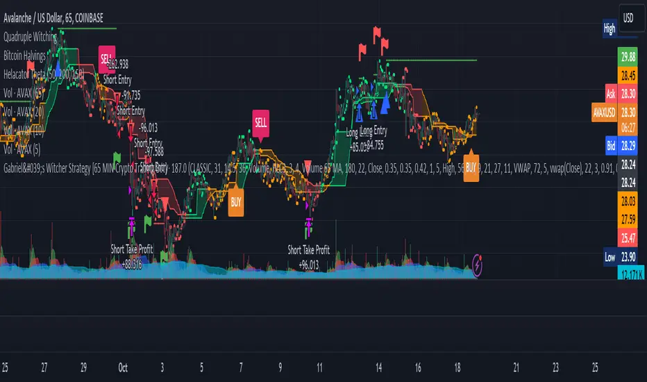
Martingale with MACD+KDJ opening conditionsStrategy Overview:
This strategy is based on a Martingale trading approach, incorporating MACD and KDJ indicators. It features pyramiding, trailing stops, and dynamic profit-taking mechanisms, suitable for both long and short trades. The strategy increases position size progressively using a Multiplier, a key feature of Martingale systems.
Key Concepts:
Martingale Strategy: A trading system where positions are doubled or increased after a loss to recover previous losses with a single successful trade. In this script, the position size is incremented using a Multiplier for each addition.
Pyramiding: Allows adding to existing trades when market conditions are favorable, enhancing profitability during trends.
Settings:
Basic Inputs:
Initial Order: Defines the starting size of the position.
Default: 150.0
MACD Settings: Customize the fast, slow, and signal smoothing lengths.
Default: Fast Length: 9, Slow Length: 26, Signal Smoothing: 9
KDJ Settings: Customize the length and smoothing parameters for KDJ.
Default: Length: 14, Smooth K: 3, Smooth D: 3
Max Additions: Sets the number of additional positions (pyramiding).
Default: 5 (Min: 1, Max: 10)
Position Sizing: Percent to add to positions on favorable conditions.
Default: 1.0%
Martingale Multiplier:
Add Multiplier: This value controls the scaling of additional positions according to the Martingale principle. After each loss, a new position is added, and its size is increased by the Multiplier factor. For example, with a multiplier of 2, each new addition will be twice as large as the previous one, accelerating recovery if the price moves favorably.
Default: 1.0 (no multiplication)
Can be adjusted up to 10x to aggressively increase position size after losses.
Trade Execution:
Long Trades:
Entry Condition: A long position is opened when the MACD line crosses over the signal line, and the KDJ’s %K crosses above %D.
Additions (Martingale): After the initial long position, new positions are added if the price drops by the defined percentage, and each new addition is increased using the Multiplier. This continues up to the set Max Additions.
Short Trades:
Entry Condition: A short position is opened when the MACD line crosses under the signal line, and the KDJ’s %K crosses below %D.
Additions (Martingale): After the initial short position, new positions are added if the price rises by the defined percentage, and each new addition is increased using the Multiplier.
Exit Conditions:
Take Profit: Exits are triggered when the price reaches the take-profit threshold.
Stop Loss: If the price moves unfavorably, the position will be closed at the set stop-loss level.
Trailing Stop: Adjusts dynamically as the price moves in favor of the trade to lock in profits.
On-Chart Visuals:
Long Signals: Blue triangles below the bars indicate long entries, and green triangles mark additional long positions.
Short Signals: Red triangles above the bars indicate short entries, and orange triangles mark additional short positions.
Information Table:
The strategy displays a table with key metrics:
Open Price: The entry price of the trade.
Average Price: The average price of the current position.
Additions: The number of additional positions taken.
Next Add Price: The price level for the next position.
Take Profit: The price at which profits will be taken.
Stop Loss: The stop-loss level to minimize risk.
Usage Instructions:
Adjust the parameters to your trading style using the input settings.
The Multiplier amplifies your position size after each addition, so use it cautiously, especially in volatile markets.
Monitor the signals and table on the chart for entry/exit decisions and trade management.

Advanced Trend Strategy [BITsPIP]The BITsPIP team is super excited to share our latest trading gem with you all. We're all about diving deep and ensuring our strategies can stand the test of time. So, we invite you to join us in exploring the awesome potential of this new strategy and really put it through its pace with some deep backtesting. This isn't just another strategy; it boasts a profit factor hovering around 1.5 across over 1000 trades, which is quite an achievement. Consider integrating it with your trading bots to further enhance your trading efficiency and profit generation. Curious? Ask for trial access or drop by our website for more details.
I. Deep Backtesting
We're all in on transparency and solid results, which is why we didn't stop at 100... or even 500 trades. We went over 1000, making sure this strategy is as robust as they come. No flimsy forecasts or sneaky repainting here. Just good, solid strategy that's ready for the real deal. Curious about the details? Check out our detailed backtesting screenshot for the BINANCE:BTCUSDT in a 5-minute timeframe. It's all about giving you the clear picture.
#No Overfitting
#No Repainting
Backtesting Screenshot
II. Algorithmic Trading
Thinking of trading as a manual game? Think again! Manual trading is a bit like rolling the dice - fun, but kind of risky if you're aiming for consistent wins. Instead, why not lean into the future with algorithmic trading? It's all about trusting the market's rhythm over the long term. By integrating your strategy with a trading bot, you can enjoy peace of mind, rest easy, and keep those emotional trades at bay.
III) Applications
Dive into the Advanced Trend Strategy, your versatile tool for navigating the market's waters. This strategy shines in under an hour timeframes, offering adaptability across stocks, commodities, forex, and cryptocurrencies. Initially fine-tuned for low-volatility cryptos like BINANCE:BTCUSDT , its default settings are a solid starting point.
But here's where your expertise comes into play. Each market beats to its own drum, necessitating nuanced adjustments to stop loss and take profit settings. This customization is key to maximizing the strategy's effectiveness in your chosen arena.
IV) Strategy's Logic
The Advanced Trend Strategy is a powerhouse, blending the precision of Hull Suite, RSI, and our unique trend detector technique. At its core, it’s designed for savvy risk management, aiming to lock in substantial profits while steering clear of minor market ripples. It utilizes stop-loss and take-profit thresholds to form a profit channel, providing a safety net for each trade. This is a trend-following strategy at heart, where these profit channels play a critical role in maximizing returns by securing positions within these "warranty channels."
1. Trend-Following
The market's complexity, influenced by countless factors, makes small movements seem almost chaotic. Yet, the principle of #Trend-Following shines in less volatile markets in long term. The strategy excels by pinpointing the ideal moments to enter the market, coupled with refined risk management to secure profits. It’s tailored for you, the individual trader, enabling you to ride the waves of market trends upwards or downwards.
2. Risk Management
A key facet of the strategy is its emphasis on pragmatic risk management. Traders are empowered to establish practical stop-loss and take-profit levels, tailoring these crucial parameters to the specific market they are engaging in. This customization is instrumental in optimizing long-term profitability, ensuring that the strategy adapts fluidly to the unique characteristics and volatility patterns of different trading environments.
V) Strategy's Input Settings and Default Values
1. Alerts
The strategy comes equipped with a flexible alert system designed to keep you informed and ready to act. Within the settings, you’ll find options to configure order/exit and comment/alert messages to your preference. This feature is particularly useful for staying on top of the strategy’s activities without constant manual oversight.
2. Hull Suite
i. Hull Suite Length: Designed for capturing long-term trends, the Hull Suite Length is configured at 1000. Functioning comparably to moving averages, the Hull Suite features upper and lower bands. Currently, it is set to 1000.
ii. Length Multiplier: It's advisable to maintain a minimal value for the Length Multiplier, prioritizing the optimization of the Hull Suite Length. Presently, it is set to 1.
3. RSI Indicator
i. The RSI is a widely recognized tool in trading. Adapt the oversold and overbought thresholds to better match the specifics of your market for optimal results.
4. StopLoss and TakeProfit
i. StopLoss and TakeProfit Settings: Two distinct approaches are available. Semi-Automatic StopLoss/TakeProfit Setting and Manual StopLoss/TakeProfit Setting. The Semi-Automatic mode streamlines the process by allowing you to input values for a 5-minute timeframe, subsequently auto-adjusting these values across various timeframes, both lower and higher. Conversely, the Manual mode offers full control, enabling you to meticulously define TakeProfit values for each individual timeframe.
ii. TakeProfit Threshold # and TakeProfit Value #: Imagine this mechanism as an ascending staircase. Each step represents a range, with the lower boundary (TakeProfit Value) designed to close the trade upon being reached, and the upper boundary (TakeProfit Threshold) upon being hit, propelling the trade to the next level, and forming a new range. This stair-stepping approach enhances risk management and increases profitability. The pre-set configurations are tailored for $BINANCE:BTCUSDT. It's advisable to devote time to tailoring these settings to your specific market, aiming to achieve optimal results based on backtesting.
iii. StopLoss Value: In line with its name, this value marks the limit of loss you're prepared to accept should the market trend go against your expectations. It's crucial to note that once your asset reaches the first TakeProfit range, the initial StopLoss value becomes obsolete, supplanted by the first TakeProfit Value. The default StopLoss value is pegged at 1.6(%), a figure worth considering in your trading strategy.
VI) Entry Conditions
The primary signal for entry is generated by our custom trend detection mechanism and hull suite values (ascending/descending). This is supported by additional indicators acting as confirmation.
VII) Exit Conditions
The strategy stipulates exit conditions primarily governed by stop loss and take profit parameters. On infrequent occasions, if the trend lacks confirmation post-entry, the strategy mandates an exit upon the issuance of a reverse signal (whether confirmed or unconfirmed) by the strategy itself.
BITsPIP

Machine Learning: SuperTrend Strategy TP/SL [YinYangAlgorithms]The SuperTrend is a very useful Indicator to display when trends have shifted based on the Average True Range (ATR). Its underlying ideology is to calculate the ATR using a fixed length and then multiply it by a factor to calculate the SuperTrend +/-. When the close crosses the SuperTrend it changes direction.
This Strategy features the Traditional SuperTrend Calculations with Machine Learning (ML) and Take Profit / Stop Loss applied to it. Using ML on the SuperTrend allows for the ability to sort data from previous SuperTrend calculations. We can filter the data so only previous SuperTrends that follow the same direction and are within the distance bounds of our k-Nearest Neighbour (KNN) will be added and then averaged. This average can either be achieved using a Mean or with an Exponential calculation which puts added weight on the initial source. Take Profits and Stop Losses are then added to the ML SuperTrend so it may capitalize on Momentum changes meanwhile remaining in the Trend during consolidation.
By applying Machine Learning logic and adding a Take Profit and Stop Loss to the Traditional SuperTrend, we may enhance its underlying calculations with potential to withhold the trend better. The main purpose of this Strategy is to minimize losses and false trend changes while maximizing gains. This may be achieved by quick reversals of trends where strategic small losses are taken before a large trend occurs with hopes of potentially occurring large gain. Due to this logic, the Win/Loss ratio of this Strategy may be quite poor as it may take many small marginal losses where there is consolidation. However, it may also take large gains and capitalize on strong momentum movements.
Tutorial:
In this example above, we can get an idea of what the default settings may achieve when there is momentum. It focuses on attempting to hit the Trailing Take Profit which moves in accord with the SuperTrend just with a multiplier added. When momentum occurs it helps push the SuperTrend within it, which on its own may act as a smaller Trailing Take Profit of its own accord.
We’ve highlighted some key points from the last example to better emphasize how it works. As you can see, the White Circle is where profit was taken from the ML SuperTrend simply from it attempting to switch to a Bullish (Buy) Trend. However, that was rejected almost immediately and we went back to our Bearish (Sell) Trend that ended up resulting in our Take Profit being hit (Yellow Circle). This Strategy aims to not only capitalize on the small profits from SuperTrend to SuperTrend but to also capitalize when the Momentum is so strong that the price moves X% away from the SuperTrend and is able to hit the Take Profit location. This Take Profit addition to this Strategy is crucial as momentum may change state shortly after such drastic price movements; and if we were to simply wait for it to come back to the SuperTrend, we may lose out on lots of potential profit.
If you refer to the Yellow Circle in this example, you’ll notice what was talked about in the Summary/Overview above. During periods of consolidation when there is little momentum and price movement and we don’t have any Stop Loss activated, you may see ‘Signal Flashing’. Signal Flashing is when there are Buy and Sell signals that keep switching back and forth. During this time you may be taking small losses. This is a normal part of this Strategy. When a signal has finally been confirmed by Momentum, is when this Strategy shines and may produce the profit you desire.
You may be wondering, what causes these jagged like patterns in the SuperTrend? It's due to the ML logic, and it may be a little confusing, but essentially what is happening is the Fast Moving SuperTrend and the Slow Moving SuperTrend are creating KNN Min and Max distances that are extreme due to (usually) parabolic movement. This causes fewer values to be added to and averaged within the ML and causes less smooth and more exponential drastic movements. This is completely normal, and one of the perks of using k-Nearest Neighbor for ML calculations. If you don’t know, the Min and Max Distance allowed is derived from the most recent(0 index of data array) to KNN Length. So only SuperTrend values that exhibit distances within these Min/Max will be allowed into the average.
Since the KNN ML logic can cause these exponential movements in the SuperTrend, they likewise affect its Take Profit. The Take Profit may benefit from this movement like displayed in the example above which helped it claim profit before then exhibiting upwards movement.
By default our Stop Loss Multiplier is kept quite low at 0.0000025. Keeping it low may help to reduce some Signal Flashing while not taking extra losses more so than not using it at all. However, if we increase it even more to say 0.005 like is shown in the example above. It can really help the trend keep momentum. Please note, although previous results don’t imply future results, at 0.0000025 Stop Loss we are currently exhibiting 69.27% profit while at 0.005 Stop Loss we are exhibiting 33.54% profit. This just goes to show that although there may be less Signal Flashing, it may not result in more profit.
We will conclude our Tutorial here. Hopefully this has given you some insight as to how Machine Learning, combined with Trailing Take Profit and Stop Loss may have positive effects on the SuperTrend when turned into a Strategy.
Settings:
SuperTrend:
ATR Length: ATR Length used to create the Original Supertrend.
Factor: Multiplier used to create the Original Supertrend.
Stop Loss Multiplier: 0 = Don't use Stop Loss. Stop loss can be useful for helping to prevent false signals but also may result in more loss when hit and less profit when switching trends.
Take Profit Multiplier: Take Profits can be useful within the Supertrend Strategy to stop the price reverting all the way to the Stop Loss once it's been profitable.
Machine Learning:
Only Factor Same Trend Direction: Very useful for ensuring that data used in KNN is not manipulated by different SuperTrend Directional data. Please note, it doesn't affect KNN Exponential.
Rationalized Source Type: Should we Rationalize only a specific source, All or None?
Machine Learning Type: Are we using a Simple ML Average, KNN Mean Average, KNN Exponential Average or None?
Machine Learning Smoothing Type: How should we smooth our Fast and Slow ML Datas to be used in our KNN Distance calculation? SMA, EMA or VWMA?
KNN Distance Type: We need to check if distance is within the KNN Min/Max distance, which distance checks are we using.
Machine Learning Length: How far back is our Machine Learning going to keep data for.
k-Nearest Neighbour (KNN) Length: How many k-Nearest Neighbours will we account for?
Fast ML Data Length: What is our Fast ML Length?? This is used with our Slow Length to create our KNN Distance.
Slow ML Data Length: What is our Slow ML Length?? This is used with our Fast Length to create our KNN Distance.
If you have any questions, comments, ideas or concerns please don't hesitate to contact us.
HAPPY TRADING!
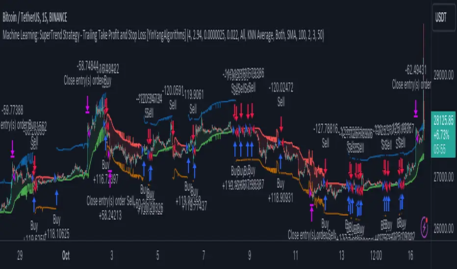
GKD-BT Full Giga Kaleidoscope Backtest [Loxx]Giga Kaleidoscope GKD-BT Full Giga Kaleidoscope Backtest is a Backtesting module included in Loxx's "Giga Kaleidoscope Modularized Trading System".
█ GKD-BT Full Giga Kaleidoscope Backtest
The Full Giga Kaleidoscope Backtest module enables users to backtest Full GKD Long and Short signals, allowing the creation of a comprehensive NNFX trading system consisting of two confirmation indicators, a baseline, a measure of volatility/volume, and continuations.
This module offers two types of backtests: Trading and Full. The Trading backtest allows users to evaluate individual Long and Short trades one by one. On the other hand, the Full backtest enables the analysis of Longs or Shorts separately by toggling between them in the settings, providing insights into the results for each signal type. The Trading backtest simulates actual trading conditions, while the Full backtest evaluates all signals regardless of their Long or Short nature.
Additionally, the backtest module allows testing with 1 to 3 take profits and 1 stop loss. The Trading backtest supports 1 to 3 take profits, while the Full backtest is limited to 1 take profit. The Trading backtest also includes a trailing take profit feature.
Regarding the percentage of trade removed at each take profit, the backtest module incorporates the following predefined values:
Take profit 1: 50% of the trade is removed.
Take profit 2: 25% of the trade is removed.
Take profit 3: 25% of the trade is removed.
Stop loss: 100% of the trade is removed.
After achieving each take profit, the stop loss level is adjusted accordingly. When take profit 1 is reached, the stop loss is moved to the entry point. Similarly, when take profit 2 is reached, the stop loss is shifted to take profit 1. The trailing take profit feature comes into effect after take profit 2 or take profit 3, depending on the number of take profits selected in the settings. The trailing take profit is always activated on the final take profit when 2 or more take profits are chosen.
The backtest module also provides the option to restrict testing to a specific date range, allowing for simulated forward testing using past data. Additionally, users can choose to display or hide a trading panel that provides relevant information about the backtest, statistics, and the current trade. It is also possible to activate alerts and toggle sections of the trading panel on or off. Historical take profit and stop loss levels are displayed as overlaid horizontal lines on the chart for reference.
To utilize this strategy, follow these steps:
1. GKD-B Baseline Import: Import the value "Input into NEW GKD-BT Backtest" from the GKD-B Baseline module into the GKD-BT Full Giga Kaleidoscope Backtest module setting named "Import GKD-B Baseline."
2. GKD-V Volatility/Volume Import: Import the value "Input into NEW GKD-BT Backtest" from the GKD-V Volatility/Volume module into the GKD-BT Full Giga Kaleidoscope Backtest module setting named "Import GKD-V Volatility/Volume."
3. Adjust the "Confirmation 1 Type" in the GKD-C Confirmation Indicator to "GKD New."
4. GKD-C Confirmation 1 Import: Import the value "Input into NEW GKD-BT Backtest" from the GKD-C Confirmation 1 module into the GKD-BT Full Giga Kaleidoscope Backtest module setting named "Import GKD-C Confirmation 1."
5. Adjust the "Confirmation 2 Type" in the GKD-C Confirmation 2 Indicator to "GKD New."
6. GKD-C Confirmation 2 Import: Import the value "Input into NEW GKD-BT Backtest" from the GKD-C Confirmation 2 module into the GKD-BT Full Giga Kaleidoscope Backtest module setting named "Import GKD-C Confirmation 2."
7. Adjust the "Confirmation Type" in the GKD-C Continuation Indicator to "GKD New."
8. GKD-C Continuation Import: Import the value "Input into NEW GKD-BT Backtest" from the GKD-C Continuation module into the GKD-BT Full Giga Kaleidoscope Backtest module setting named "Import GKD-C Confirmation."
The GKD system utilizes volatility-based take profits and stop losses, where each take profit and stop loss is calculated as a multiple of volatility. Users have the flexibility to adjust the multiplier values in the settings to suit their preferences.
In a future update, the Full Giga Kaleidoscope Backtest module will include the option to incorporate a GKD-E Exit indicator, completing the full trading strategy.
█ Full Giga Kaleidoscope Backtest Entries
Within this module, there are ten distinct types of entries available, which are outlined below:
Standard Entry
1-Candle Standard Entry
Baseline Entry
1-Candle Baseline Entry
Volatility/Volume Entry
1-Candle Volatility/Volume Entry
Confirmation 2 Entry
1-Candle Confirmation 2 Entry
PullBack Entry
Continuation Entry
Each of these entry types can generate either long or short signals, resulting in a total of 20 signal variations. The user has the flexibility to enable or disable specific entry types and choose which qualifying rules within each entry type are applied to price to determine the final long or short signal.
The following section provides an overview of the various entry types and their corresponding qualifying rules:
Standard Entry
1. GKD-C Confirmation gives signal
2. Baseline agrees
3. Price inside Goldie Locks Zone Minimum
4. Price inside Goldie Locks Zone Maximum
5. Confirmation 2 agrees
6. Volatility/Volume agrees
1-Candle Standard Entry
1a. GKD-C Confirmation gives signal
2a. Baseline agrees
3a. Price inside Goldie Locks Zone Minimum
4a. Price inside Goldie Locks Zone Maximum
Next Candle
1b. Price retraced
2b. Baseline agrees
3b. Confirmation 1 agrees
4b. Confirmation 2 agrees
5b. Volatility/Volume agrees
Baseline Entry
1. GKD-B Basline gives signal
2. Confirmation 1 agrees
3. Price inside Goldie Locks Zone Minimum
4. Price inside Goldie Locks Zone Maximum
5. Confirmation 2 agrees
6. Volatility/Volume agrees
7. Confirmation 1 signal was less than 'Maximum Allowable PSBC Bars Back' prior
1-Candle Baseline Entry
1a. GKD-B Baseline gives signal
2a. Confirmation 1 agrees
3a. Price inside Goldie Locks Zone Minimum
4a. Price inside Goldie Locks Zone Maximum
5a. Confirmation 1 signal was less than 'Maximum Allowable PSBC Bars Back' prior
Next Candle
1b. Price retraced
2b. Baseline agrees
3b. Confirmation 1 agrees
4b. Confirmation 2 agrees
5b. Volatility/Volume agrees
Volatility/Volume Entry
1. GKD-V Volatility/Volume gives signal
2. Confirmation 1 agrees
3. Price inside Goldie Locks Zone Minimum
4. Price inside Goldie Locks Zone Maximum
5. Confirmation 2 agrees
6. Baseline agrees
7. Confirmation 1 signal was less than 7 candles prior
1-Candle Volatility/Volume Entry
1a. GKD-V Volatility/Volume gives signal
2a. Confirmation 1 agrees
3a. Price inside Goldie Locks Zone Minimum
4a. Price inside Goldie Locks Zone Maximum
5a. Confirmation 1 signal was less than 'Maximum Allowable PSVVC Bars Back' prior
Next Candle
1b. Price retraced
2b. Volatility/Volume agrees
3b. Confirmation 1 agrees
4b. Confirmation 2 agrees
5b. Baseline agrees
Confirmation 2 Entry
1. GKD-C Confirmation 2 gives signal
2. Confirmation 1 agrees
3. Price inside Goldie Locks Zone Minimum
4. Price inside Goldie Locks Zone Maximum
5. Volatility/Volume agrees
6. Baseline agrees
7. Confirmation 1 signal was less than 7 candles prior
1-Candle Confirmation 2 Entry
1a. GKD-C Confirmation 2 gives signal
2a. Confirmation 1 agrees
3a. Price inside Goldie Locks Zone Minimum
4a. Price inside Goldie Locks Zone Maximum
5a. Confirmation 1 signal was less than 'Maximum Allowable PSC2C Bars Back' prior
Next Candle
1b. Price retraced
2b. Confirmation 2 agrees
3b. Confirmation 1 agrees
4b. Volatility/Volume agrees
5b. Baseline agrees
PullBack Entry
1a. GKD-B Baseline gives signal
2a. Confirmation 1 agrees
3a. Price is beyond 1.0x Volatility of Baseline
Next Candle
1b. Price inside Goldie Locks Zone Minimum
2b. Price inside Goldie Locks Zone Maximum
3b. Confirmation 1 agrees
4b. Confirmation 2 agrees
5b. Volatility/Volume agrees
Continuation Entry
1. Standard Entry, 1-Candle Standard Entry, Baseline Entry, 1-Candle Baseline Entry, Volatility/Volume Entry, 1-Candle Volatility/Volume Entry, Confirmation 2 Entry, 1-Candle Confirmation 2 Entry, or Pullback entry triggered previously
2. Baseline hasn't crossed since entry signal trigger
4. Confirmation 1 agrees
5. Baseline agrees
6. Confirmation 2 agrees
█ Volatility Types Included
This module includes 17 types of volatility:
Close-to-Close
Parkinson
Garman-Klass
Rogers-Satchell
Yang-Zhang
Garman-Klass-Yang-Zhang
Exponential Weighted Moving Average
Standard Deviation of Log Returns
Pseudo GARCH(2,2)
Average True Range
True Range Double
Standard Deviation
Adaptive Deviation
Median Absolute Deviation
Efficiency-Ratio Adaptive ATR
Mean Absolute Deviation
Static Percent
Close-to-Close
Close-to-Close volatility is a classic and widely used volatility measure, sometimes referred to as historical volatility.
Volatility is an indicator of the speed of a stock price change. A stock with high volatility is one where the price changes rapidly and with a larger amplitude. The more volatile a stock is, the riskier it is.
Close-to-close historical volatility is calculated using only a stock's closing prices. It is the simplest volatility estimator. However, in many cases, it is not precise enough. Stock prices could jump significantly during a trading session and return to the opening value at the end. That means that a considerable amount of price information is not taken into account by close-to-close volatility.
Despite its drawbacks, Close-to-Close volatility is still useful in cases where the instrument doesn't have intraday prices. For example, mutual funds calculate their net asset values daily or weekly, and thus their prices are not suitable for more sophisticated volatility estimators.
Parkinson
Parkinson volatility is a volatility measure that uses the stock’s high and low price of the day.
The main difference between regular volatility and Parkinson volatility is that the latter uses high and low prices for a day, rather than only the closing price. This is useful as close-to-close prices could show little difference while large price movements could have occurred during the day. Thus, Parkinson's volatility is considered more precise and requires less data for calculation than close-to-close volatility.
One drawback of this estimator is that it doesn't take into account price movements after the market closes. Hence, it systematically undervalues volatility. This drawback is addressed in the Garman-Klass volatility estimator.
Garman-Klass
Garman-Klass is a volatility estimator that incorporates open, low, high, and close prices of a security.
Garman-Klass volatility extends Parkinson's volatility by taking into account the opening and closing prices. As markets are most active during the opening and closing of a trading session, it makes volatility estimation more accurate.
Garman and Klass also assumed that the process of price change follows a continuous diffusion process (Geometric Brownian motion). However, this assumption has several drawbacks. The method is not robust for opening jumps in price and trend movements.
Despite its drawbacks, the Garman-Klass estimator is still more effective than the basic formula since it takes into account not only the price at the beginning and end of the time interval but also intraday price extremes.
Researchers Rogers and Satchell have proposed a more efficient method for assessing historical volatility that takes into account price trends. See Rogers-Satchell Volatility for more detail.
Rogers-Satchell
Rogers-Satchell is an estimator for measuring the volatility of securities with an average return not equal to zero.
Unlike Parkinson and Garman-Klass estimators, Rogers-Satchell incorporates a drift term (mean return not equal to zero). As a result, it provides better volatility estimation when the underlying is trending.
The main disadvantage of this method is that it does not take into account price movements between trading sessions. This leads to an underestimation of volatility since price jumps periodically occur in the market precisely at the moments between sessions.
A more comprehensive estimator that also considers the gaps between sessions was developed based on the Rogers-Satchel formula in the 2000s by Yang-Zhang. See Yang Zhang Volatility for more detail.
Yang-Zhang
Yang Zhang is a historical volatility estimator that handles both opening jumps and the drift and has a minimum estimation error.
Yang-Zhang volatility can be thought of as a combination of the overnight (close-to-open volatility) and a weighted average of the Rogers-Satchell volatility and the day’s open-to-close volatility. It is considered to be 14 times more efficient than the close-to-close estimator.
Garman-Klass-Yang-Zhang
Garman-Klass-Yang-Zhang (GKYZ) volatility estimator incorporates the returns of open, high, low, and closing prices in its calculation.
GKYZ volatility estimator takes into account overnight jumps but not the trend, i.e., it assumes that the underlying asset follows a Geometric Brownian Motion (GBM) process with zero drift. Therefore, the GKYZ volatility estimator tends to overestimate the volatility when the drift is different from zero. However, for a GBM process, this estimator is eight times more efficient than the close-to-close volatility estimator.
Exponential Weighted Moving Average
The Exponentially Weighted Moving Average (EWMA) is a quantitative or statistical measure used to model or describe a time series. The EWMA is widely used in finance, with the main applications being technical analysis and volatility modeling.
The moving average is designed such that older observations are given lower weights. The weights decrease exponentially as the data point gets older – hence the name exponentially weighted.
The only decision a user of the EWMA must make is the parameter lambda. The parameter decides how important the current observation is in the calculation of the EWMA. The higher the value of lambda, the more closely the EWMA tracks the original time series.
Standard Deviation of Log Returns
This is the simplest calculation of volatility. It's the standard deviation of ln(close/close(1)).
Pseudo GARCH(2,2)
This is calculated using a short- and long-run mean of variance multiplied by ?.
?avg(var;M) + (1 ? ?) avg(var;N) = 2?var/(M+1-(M-1)L) + 2(1-?)var/(M+1-(M-1)L)
Solving for ? can be done by minimizing the mean squared error of estimation; that is, regressing L^-1var - avg(var; N) against avg(var; M) - avg(var; N) and using the resulting beta estimate as ?.
Average True Range
The average true range (ATR) is a technical analysis indicator, introduced by market technician J. Welles Wilder Jr. in his book New Concepts in Technical Trading Systems, that measures market volatility by decomposing the entire range of an asset price for that period.
The true range indicator is taken as the greatest of the following: current high less the current low; the absolute value of the current high less the previous close; and the absolute value of the current low less the previous close. The ATR is then a moving average, generally using 14 days, of the true ranges.
True Range Double
A special case of ATR that attempts to correct for volatility skew.
Standard Deviation
Standard deviation is a statistic that measures the dispersion of a dataset relative to its mean and is calculated as the square root of the variance. The standard deviation is calculated as the square root of variance by determining each data point's deviation relative to the mean. If the data points are further from the mean, there is a higher deviation within the data set; thus, the more spread out the data, the higher the standard deviation.
Adaptive Deviation
By definition, the Standard Deviation (STD, also represented by the Greek letter sigma ? or the Latin letter s) is a measure that is used to quantify the amount of variation or dispersion of a set of data values. In technical analysis, we usually use it to measure the level of current volatility.
Standard Deviation is based on Simple Moving Average calculation for mean value. This version of standard deviation uses the properties of EMA to calculate what can be called a new type of deviation, and since it is based on EMA, we can call it EMA deviation. Additionally, Perry Kaufman's efficiency ratio is used to make it adaptive (since all EMA type calculations are nearly perfect for adapting).
The difference when compared to the standard is significant--not just because of EMA usage, but the efficiency ratio makes it a "bit more logical" in very volatile market conditions.
Median Absolute Deviation
The median absolute deviation is a measure of statistical dispersion. Moreover, the MAD is a robust statistic, being more resilient to outliers in a data set than the standard deviation. In the standard deviation, the distances from the mean are squared, so large deviations are weighted more heavily, and thus outliers can heavily influence it. In the MAD, the deviations of a small number of outliers are irrelevant.
Because the MAD is a more robust estimator of scale than the sample variance or standard deviation, it works better with distributions without a mean or variance, such as the Cauchy distribution.
Efficiency-Ratio Adaptive ATR
Average True Range (ATR) is a widely used indicator for many occasions in technical analysis. It is calculated as the RMA of the true range. This version adds a "twist": it uses Perry Kaufman's Efficiency Ratio to calculate adaptive true range.
Mean Absolute Deviation
The mean absolute deviation (MAD) is a measure of variability that indicates the average distance between observations and their mean. MAD uses the original units of the data, which simplifies interpretation. Larger values signify that the data points spread out further from the average. Conversely, lower values correspond to data points bunching closer to it. The mean absolute deviation is also known as the mean deviation and average absolute deviation.
This definition of the mean absolute deviation sounds similar to the standard deviation (SD). While both measure variability, they have different calculations. In recent years, some proponents of MAD have suggested that it replace the SD as the primary measure because it is a simpler concept that better fits real life.
Static Percent
Static Percent allows the user to insert their own constant percent that will then be used to create take profits and stoploss
█ Giga Kaleidoscope Modularized Trading System
Core components of an NNFX algorithmic trading strategy
The NNFX algorithm is built on the principles of trend, momentum, and volatility. There are six core components in the NNFX trading algorithm:
1. Volatility - price volatility; e.g., Average True Range, True Range Double, Close-to-Close, etc.
2. Baseline - a moving average to identify price trend
3. Confirmation 1 - a technical indicator used to identify trends
4. Confirmation 2 - a technical indicator used to identify trends
5. Continuation - a technical indicator used to identify trends
6. Volatility/Volume - a technical indicator used to identify volatility/volume breakouts/breakdown
7. Exit - a technical indicator used to determine when a trend is exhausted
What is Volatility in the NNFX trading system?
In the NNFX (No Nonsense Forex) trading system, ATR (Average True Range) is typically used to measure the volatility of an asset. It is used as a part of the system to help determine the appropriate stop loss and take profit levels for a trade. ATR is calculated by taking the average of the true range values over a specified period.
True range is calculated as the maximum of the following values:
-Current high minus the current low
-Absolute value of the current high minus the previous close
-Absolute value of the current low minus the previous close
ATR is a dynamic indicator that changes with changes in volatility. As volatility increases, the value of ATR increases, and as volatility decreases, the value of ATR decreases. By using ATR in NNFX system, traders can adjust their stop loss and take profit levels according to the volatility of the asset being traded. This helps to ensure that the trade is given enough room to move, while also minimizing potential losses.
Other types of volatility include True Range Double (TRD), Close-to-Close, and Garman-Klass
What is a Baseline indicator?
The baseline is essentially a moving average, and is used to determine the overall direction of the market.
The baseline in the NNFX system is used to filter out trades that are not in line with the long-term trend of the market. The baseline is plotted on the chart along with other indicators, such as the Moving Average (MA), the Relative Strength Index (RSI), and the Average True Range (ATR).
Trades are only taken when the price is in the same direction as the baseline. For example, if the baseline is sloping upwards, only long trades are taken, and if the baseline is sloping downwards, only short trades are taken. This approach helps to ensure that trades are in line with the overall trend of the market, and reduces the risk of entering trades that are likely to fail.
By using a baseline in the NNFX system, traders can have a clear reference point for determining the overall trend of the market, and can make more informed trading decisions. The baseline helps to filter out noise and false signals, and ensures that trades are taken in the direction of the long-term trend.
What is a Confirmation indicator?
Confirmation indicators are technical indicators that are used to confirm the signals generated by primary indicators. Primary indicators are the core indicators used in the NNFX system, such as the Average True Range (ATR), the Moving Average (MA), and the Relative Strength Index (RSI).
The purpose of the confirmation indicators is to reduce false signals and improve the accuracy of the trading system. They are designed to confirm the signals generated by the primary indicators by providing additional information about the strength and direction of the trend.
Some examples of confirmation indicators that may be used in the NNFX system include the Bollinger Bands, the MACD (Moving Average Convergence Divergence), and the MACD Oscillator. These indicators can provide information about the volatility, momentum, and trend strength of the market, and can be used to confirm the signals generated by the primary indicators.
In the NNFX system, confirmation indicators are used in combination with primary indicators and other filters to create a trading system that is robust and reliable. By using multiple indicators to confirm trading signals, the system aims to reduce the risk of false signals and improve the overall profitability of the trades.
What is a Continuation indicator?
In the NNFX (No Nonsense Forex) trading system, a continuation indicator is a technical indicator that is used to confirm a current trend and predict that the trend is likely to continue in the same direction. A continuation indicator is typically used in conjunction with other indicators in the system, such as a baseline indicator, to provide a comprehensive trading strategy.
What is a Volatility/Volume indicator?
Volume indicators, such as the On Balance Volume (OBV), the Chaikin Money Flow (CMF), or the Volume Price Trend (VPT), are used to measure the amount of buying and selling activity in a market. They are based on the trading volume of the market, and can provide information about the strength of the trend. In the NNFX system, volume indicators are used to confirm trading signals generated by the Moving Average and the Relative Strength Index. Volatility indicators include Average Direction Index, Waddah Attar, and Volatility Ratio. In the NNFX trading system, volatility is a proxy for volume and vice versa.
By using volume indicators as confirmation tools, the NNFX trading system aims to reduce the risk of false signals and improve the overall profitability of trades. These indicators can provide additional information about the market that is not captured by the primary indicators, and can help traders to make more informed trading decisions. In addition, volume indicators can be used to identify potential changes in market trends and to confirm the strength of price movements.
What is an Exit indicator?
The exit indicator is used in conjunction with other indicators in the system, such as the Moving Average (MA), the Relative Strength Index (RSI), and the Average True Range (ATR), to provide a comprehensive trading strategy.
The exit indicator in the NNFX system can be any technical indicator that is deemed effective at identifying optimal exit points. Examples of exit indicators that are commonly used include the Parabolic SAR, the Average Directional Index (ADX), and the Chandelier Exit.
The purpose of the exit indicator is to identify when a trend is likely to reverse or when the market conditions have changed, signaling the need to exit a trade. By using an exit indicator, traders can manage their risk and prevent significant losses.
In the NNFX system, the exit indicator is used in conjunction with a stop loss and a take profit order to maximize profits and minimize losses. The stop loss order is used to limit the amount of loss that can be incurred if the trade goes against the trader, while the take profit order is used to lock in profits when the trade is moving in the trader's favor.
Overall, the use of an exit indicator in the NNFX trading system is an important component of a comprehensive trading strategy. It allows traders to manage their risk effectively and improve the profitability of their trades by exiting at the right time.
How does Loxx's GKD (Giga Kaleidoscope Modularized Trading System) implement the NNFX algorithm outlined above?
Loxx's GKD v2.0 system has five types of modules (indicators/strategies). These modules are:
1. GKD-BT - Backtesting module (Volatility, Number 1 in the NNFX algorithm)
2. GKD-B - Baseline module (Baseline and Volatility/Volume, Numbers 1 and 2 in the NNFX algorithm)
3. GKD-C - Confirmation 1/2 and Continuation module (Confirmation 1/2 and Continuation, Numbers 3, 4, and 5 in the NNFX algorithm)
4. GKD-V - Volatility/Volume module (Confirmation 1/2, Number 6 in the NNFX algorithm)
5. GKD-E - Exit module (Exit, Number 7 in the NNFX algorithm)
(additional module types will added in future releases)
Each module interacts with every module by passing data to A backtest module wherein the various components of the GKD system are combined to create a trading signal.
That is, the Baseline indicator passes its data to Volatility/Volume. The Volatility/Volume indicator passes its values to the Confirmation 1 indicator. The Confirmation 1 indicator passes its values to the Confirmation 2 indicator. The Confirmation 2 indicator passes its values to the Continuation indicator. The Continuation indicator passes its values to the Exit indicator, and finally, the Exit indicator passes its values to the Backtest strategy.
This chaining of indicators requires that each module conform to Loxx's GKD protocol, therefore allowing for the testing of every possible combination of technical indicators that make up the six components of the NNFX algorithm.
What does the application of the GKD trading system look like?
Example trading system:
Backtest: Full Giga Kaleidoscope Backtest as shown on the chart above
Baseline: Hull Moving Average as shown on the chart above
Volatility/Volume: Hurst Exponent as shown on the chart above
Confirmation 1: Vorext as shown on the chart above
Confirmation 2: Coppock Curve as shown on the chart above
Continuation: Fisher Transform as shown on the chart above
Exit: Rex Oscillator
Each GKD indicator is denoted with a module identifier of either: GKD-BT, GKD-B, GKD-C, GKD-V, or GKD-E. This allows traders to understand to which module each indicator belongs and where each indicator fits into the GKD system.